3D Ising Model with Parallel Computing

Introduction

Background

Ferromagnetism and phase transitions are fundamental concepts in statistical mechanics. The Ising Model provides a simplified yet effective framework to study these phenomena by modeling spins on a lattice. This report focuses on a 3D Ising Model and its application to high-dimensional problems.

The Ising model, first proposed by Wilhelm Lenz in 1920 and solved by his student Ernst Ising in 1D, has become one of the most important models in statistical physics. It successfully describes ferromagnetic-paramagnetic phase transitions and serves as a paradigm for understanding critical phenomena.

In ferromagnetic materials, atomic spins tend to align parallel to each other below a critical temperature (Curie temperature), resulting in spontaneous magnetization. Above this temperature, thermal fluctuations overcome the alignment tendency, leading to a paramagnetic phase. The 3D Ising model captures this behavior through nearest-neighbor interactions on a cubic lattice.

Objective

The goal of this project is to simulate the 3D Ising Model using parallel computing approaches, leveraging MPI for distributed memory and GPUs for acceleration. Special emphasis is placed on scalability, performance optimization, and future enhancements. I aim to:

• Implement and analyze the 3D Ising model below its critical temperature
• Study finite-size scaling effects in large systems
• Develop efficient parallel algorithms for spin updates and energy calculations
• Compare different optimization strategies for high-performance computing

Theoretical Background

Ising Model Formulation

The Ising Model represents spins on a lattice, each taking a value of +1 or -1. From physics, I know that the system will minimize the Hamiltonian. The Hamiltonian is defined as:

where J is the interaction strength, h is the external magnetic field, and s_i denotes the spin at site i. The notation ⟨i,j⟩ indicates summation over nearest neighbors only. In my 3D implementation, each lattice site has six nearest neighbors (±x, ±y, ±z directions).

The energy change for a single spin flip is given by:

where the sum runs over nearest neighbors of site i. This local energy change ΔE is crucial for the Metropolis algorithm implementation.

Monte Carlo Simulation

Monte Carlo methods are essential for studying the 3D Ising model because they provide a way to sample the enormous configuration space efficiently. With 2^N possible states for N spins, direct enumeration becomes impossible for any reasonably sized system. The Metropolis-Hastings algorithm, a Markov Chain Monte Carlo (MCMC) method, allows me to generate configurations with probability proportional to the Boltzmann distribution exp(-E/k_BT).

The Metropolis algorithm is employed for simulation. The algorithm proceeds as follows:

For each Monte Carlo step:
  1. Select random lattice site (i,j,k)
  2. s_old ← spin at (i,j,k)
  3. Calculate ΔE = -s_old(J∑_neighbors s_n + h)
  4. If ΔE ≤ 0:
       Flip spin: s_new = -s_old
     Else:
       Generate random number r ∈ [0,1]
       If r < min(1, exp(-ΔE/k_BT)):
         Flip spin: s_new = -s_old

Each Monte Carlo step involves attempting to flip individual spins and accepting or rejecting these moves based on the energy change ΔE. The acceptance probability follows the Metropolis criterion:

This approach allows the system to:

• Always accept moves that lower the energy (ΔE < 0)
• Sometimes accept moves that increase the energy, with probability decreasing exponentially with ΔE
• Maintain thermal fluctuations appropriate for the temperature T
• Eventually reach thermal equilibrium

Serial Implementation

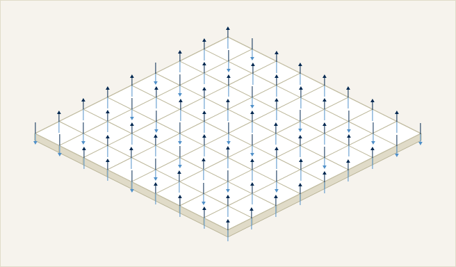
The serial implementation utilizes the sweeping method to systematically update spins across the lattice. To enhance statistical reliability, a red-black update scheme is applied, which alternates updates between subsets of spins to prevent pattern formation. Without this, I get pattern formation. In particular, when the size of the lattice is even, I get a checkerboard pattern. While the algorithm appears to work for an odd size, I would like to build a generalized algorithm that works regardless of dimensions.

The red-black scheme divides the lattice points into two groups, like a 3D checkerboard pattern. Points (i,j,k) are classified as "red" if (i+j+k) is even, and "black" if (i+j+k) is odd. This ensures that no adjacent spins are updated simultaneously, maintaining the validity of the energy calculations.

For each Monte Carlo step:
  // Update red sites (i+j+k even)
  For all sites where (i+j+k) mod 2 = 0:
      Calculate ΔE = -s_{i,j,k}(J∑_neighbors s_n + h)
      If ΔE ≤ 0 or r < exp(-ΔE/k_BT):
          s_{i,j,k} ← -s_{i,j,k}
  
  // Update black sites (i+j+k odd)  
  For all sites where (i+j+k) mod 2 = 1:
      Calculate ΔE = -s_{i,j,k}(J∑_neighbors s_n + h)
      If ΔE ≤ 0 or r < exp(-ΔE/k_BT):
          s_{i,j,k} ← -s_{i,j,k}

This approach allows for parallel updates within each color group, which is crucial for the scalability of the simulation.

Parallelization Approaches

MPI Domain Decomposition

The parallel implementation employs a domain decomposition strategy where the 3D lattice is divided into smaller sub-domains, each handled by a separate MPI process. This decomposition maintains load balance while minimizing communication overhead. The global L × L × L lattice is partitioned into P_x × P_y × P_z sub-domains, where P_x · P_y · P_z = P (total number of processes).

Each sub-domain includes ghost layers that store copies of neighboring spins required for energy calculations. These ghost regions are updated through halo exchanges between adjacent processes after each Monte Carlo sweep. The halo exchange pattern follows a six-way communication scheme, corresponding to the six faces of each 3D sub-domain.

MPI Implementation Details

1. Create 3D Cartesian communicator with periodic boundaries
2. Divide L×L×L lattice into local domains with ghost layers
3. Initialize local spins randomly
For each Monte Carlo step:
  // Red-Black Update Pattern
  For color in {red, black}:
      For each local site (i,j,k) of current color:
          Calculate ΔE from 6 nearest neighbors
          If ΔE ≤ 0 or random < exp(-ΔE/k_BT):
              Flip spin: s_{i,j,k} ← -s_{i,j,k}
      Perform 6-way halo exchange with neighbors
  Calculate local energy and magnetization
  MPI_Reduce to get global observables
  If time to save:
      Gather lattice data to rank 0
      Write configuration to file (rank 0)

1. Pack boundary data into send buffers
For direction in {x, y, z}:
  2. MPI_Sendrecv with negative neighbor
  3. MPI_Sendrecv with positive neighbor
4. Update ghost layers with received data

The domain decomposition approach enables efficient parallel scaling by evenly distributing the work across the processes. As I see in the results, this leads to a nearly linear scaling of the runtime.

GPU Implementation

The GPU implementation leverages massive parallelism by mapping the lattice updates to the GPU's thread hierarchy. The implementation uses a block-based approach where each thread block handles a portion of the lattice, with shared memory optimizations to reduce global memory access.

This approach is combined with MPI to achieve high performance. The lattice is first decomposed across MPI processes as described in the previous section. Then, each process offloads its local computation to a GPU. The GPU kernels handle the spin updates and energy calculations, while MPI manages the inter-process communication for halo exchanges.

Implementation Limitations

There are, however, clear limitations with this basic implementation. The algorithm requires transferring data between the CPU and GPU multiple times during halo exchanges, as these are performed on the CPU. This represents a significant bottleneck in the computation. While functional, this naive approach leaves room for optimization through techniques like GPU-aware MPI and asynchronous operations.

Optimizations

My optimization journey involved three major breakthroughs that dramatically improved performance:

Precomputed Random Numbers

Problem Identified: Initial profiling revealed that random number generation was consuming approximately 60% of the total runtime, particularly in the GPU implementation. In the original implementation, random numbers were generated serially on the CPU and transferred to the GPU for each Monte Carlo step.

Solution Implemented: I migrated to cuRAND for GPU-based random number generation. Each GPU thread maintains its own random number state using cuRAND's state-based generators, allowing for parallel generation of random numbers directly on the device.

Results: The optimization reduced the time spent on random number generation from approximately 60% of the total runtime to less than 5%. This dramatic improvement stems from both the parallel generation capability and the elimination of PCIe transfers for random numbers.

Shared Memory Optimization

Problem Identified: My initial GPU implementation accessed global memory frequently, particularly during energy calculations where each spin needs to read its six nearest neighbors. This resulted in high memory latency and reduced performance.

Solution Implemented: I implemented two key shared memory strategies:

1. Block-level Loading: Thread blocks cooperatively load lattice sections into shared memory
2. Two-level Reduction: Local reduction in shared memory before global atomic operations

Results: These shared memory optimizations reduced the time to compute 1000 steps on a 64³ lattice from 0.95 to 0.71 seconds.

GPU-Aware MPI

Problem Identified: Halo exchanges required a three-step process: copying data from GPU to CPU, performing MPI communication, then copying data back to GPU. This approach introduced significant overhead.

Solution Implemented: I implemented GPU-aware MPI, which allows direct GPU-to-GPU communication between nodes. When available, this feature enables MPI to access GPU memory directly, eliminating the need for explicit CPU staging buffers.

Results: With this optimization, I brought the time to compute 1000 steps on 64³ down to 0.28 seconds.

Performance Analysis

Runtime Comparison

Below is a table of the runtime comparison across different implementations. All GPU implementations use 8 ranks.

Notably, I get a similar runtime for the MPI implementation with 1 rank and the serial implementation. With 8 ranks, I get a significant speedup of about eightfold. My naive GPU implementation is much faster than the MPI implementation, but the optimized GPU implementation is faster still. Additionally, I see good scaling with the GPU implementation, as analyzed later.

Roofline Model

The roofline model analysis provides valuable insights into the performance characteristics and limitations of my different implementations.

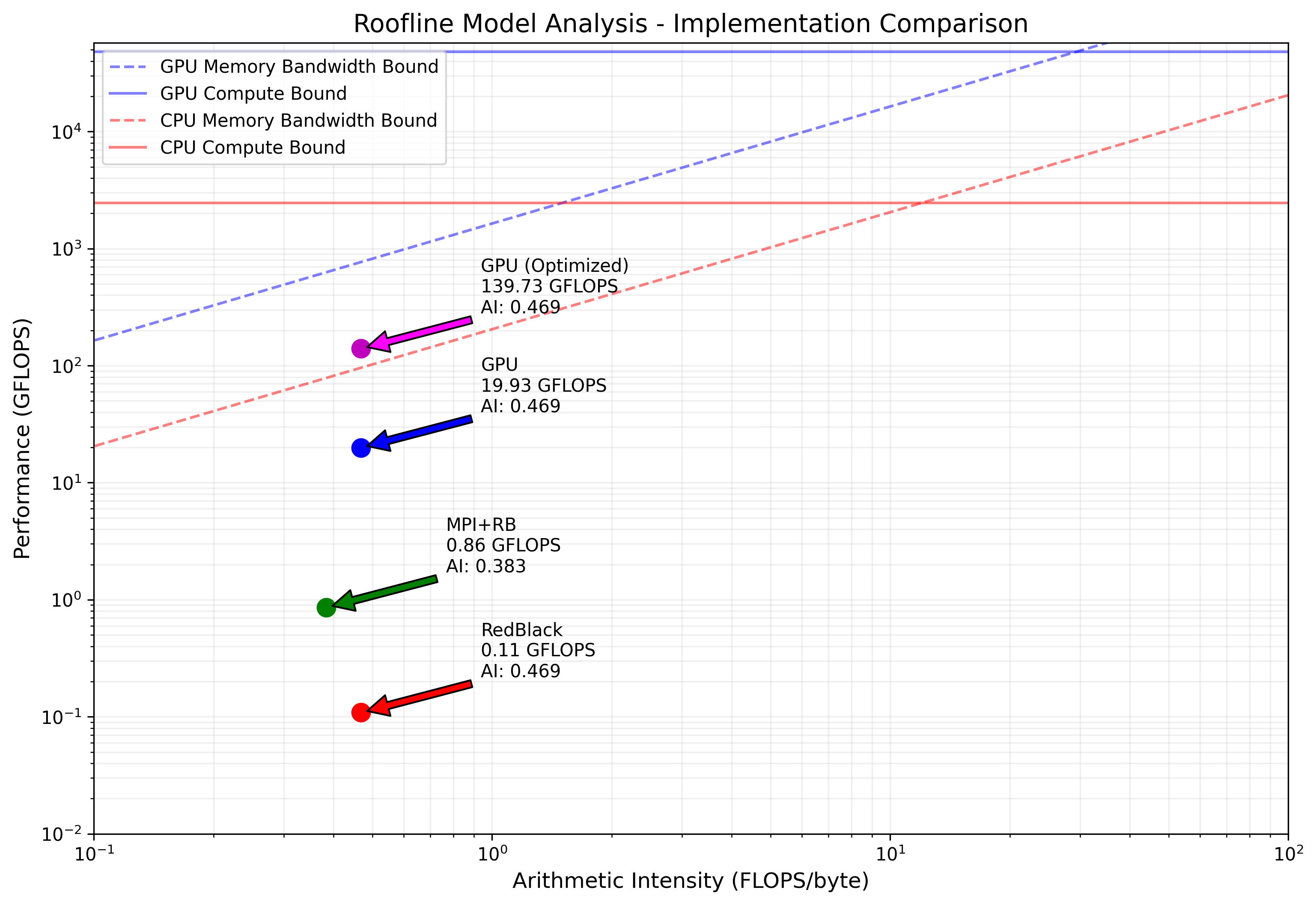
My analysis reveals that all implementations are memory-bound, operating well below their respective ridge points (AMD MI250X GPU: 29.2 FLOPS/byte, AMD EPYC 7V13 CPU: 12.0 FLOPS/byte). This is expected given the nature of the Ising model computation, where each spin update requires reading multiple neighboring values but performs relatively few arithmetic operations.

The baseline GPU implementation achieves 19.93 GFLOPS with a memory bandwidth utilization of 42.52 GB/s. However, my optimized GPU implementation shows significant improvement, reaching 139.73 GFLOPS and 298.09 GB/s memory bandwidth, approximately a 7x performance increase.

The RedBlack CPU implementation operates at 0.11 GFLOPS with a memory bandwidth of 0.23 GB/s, while the MPI+RedBlack version achieves 0.86 GFLOPS and 2.24 GB/s memory bandwidth. Both CPU implementations show relatively low hardware utilization, suggesting potential for further optimization.

Scalability

Performance is evaluated across varying lattice sizes (64³ and 256³). Looking at my results, I see my optimized GPU implementation take 0.28s for a lattice size of 64³ and 5.5s for a lattice size of 256³.

While this is a 64x increase in lattice size, I only have a ~19.6x increase in runtime. This is a clear indication of my parallelization successfully scaling and improving at scale.

Implementation Comparison

My performance analysis reveals significant differences between implementations:

• Serial vs. MPI: The single-rank MPI implementation performs similarly to the serial version (36.2s vs 35.6s), but scaling to 8 ranks yields a near-linear speedup, reducing runtime to 5.8s. This demonstrates effective parallelization with minimal overhead.

• CPU vs. GPU: The baseline GPU implementation outperforms both serial and MPI versions significantly, completing the same workload in 0.95s. This represents a 38x speedup over serial and 6.1x over 8-rank MPI implementation.

• Optimized GPU: My optimizations (shared memory, GPU-aware MPI, precomputed random numbers) further reduced the GPU runtime to 0.28s, achieving a 129x speedup over serial and a 3.4x improvement over the baseline GPU implementation.

• Scaling Behavior: When increasing the problem size from 64³ to 256³ (64x more lattice points), the optimized GPU implementation shows excellent scaling, with runtime increasing only by a factor of 19.6 (from 0.28s to 5.5s).

The efficiency analysis shows that my optimized GPU implementation achieves the highest hardware utilization, though still well below theoretical peaks due to the memory-bound nature of the algorithm. The MPI implementation demonstrates good scaling but is limited by the AMD EPYC 7V13 CPU memory bandwidth, while the GPU implementations benefit from the significantly higher memory bandwidth available on the AMD MI250X GPU accelerator.

Results

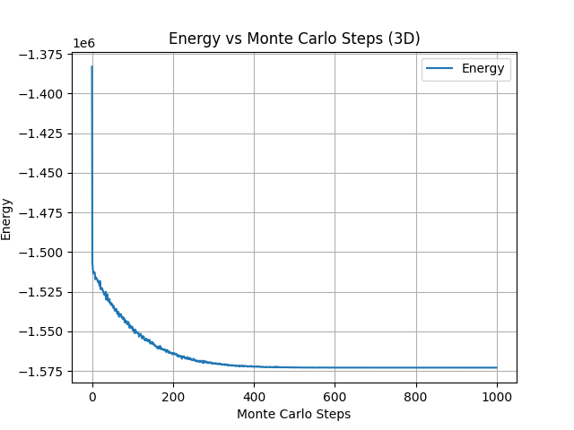
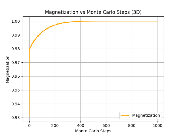
Energy and Magnetization

The energy and magnetization are plotted as functions of iteration count, demonstrating the convergence of the solution.

Visualization

In addition to metadata, such as the energy and magnetization, I can also visualize the spins on the lattice.

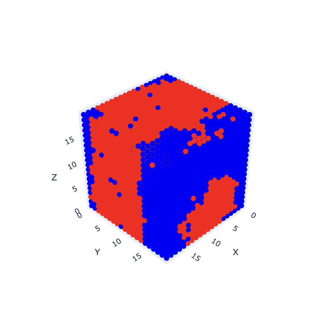
An interactive web demo can be found at https://tajgillin.neocities.org/redblack/rb. Click on the red/blue key in the top right to toggle the spin visibility!

Discussion

The implementation and analysis of the 3D Ising model reveals several key insights about parallel computing strategies and their effectiveness. My results demonstrate that while both MPI and GPU implementations offer significant performance improvements over the serial version, the optimized GPU implementation provides the best performance, achieving a 129x speedup over the serial implementation.

Key Findings

• Red-black update scheme successfully prevents pattern formation and enables parallel updates, proving essential for both MPI and GPU implementations
• Memory access patterns significantly impact performance, as shown by the substantial improvements achieved through shared memory optimizations and GPU-aware MPI
• Roofline analysis reveals that all implementations are memory-bound, suggesting that future optimizations should focus on improving memory access patterns rather than computational efficiency
• Excellent scaling behavior of my optimized GPU implementation (19.6x increase in runtime for a 64x increase in problem size) indicates effective parallelization

From a physics perspective, this simulation is being run at low temperature, and I am seeing spontaneous polarization! At high temperatures, I simply see thermal fluctuations. The visual demo is quite fun to play with.

Future Directions

Pinned Memory

One promising avenue for optimization involves the implementation of pinned memory for GPU operations. Currently, my implementation uses pageable host memory for CPU-GPU transfers, which requires the CUDA driver to first copy the data to a temporary pinned buffer before transfer. By directly allocating pinned memory, I can eliminate this extra copy and achieve higher bandwidth for memory transfers.

Asynchronous Streams

A significant optimization opportunity lies in the implementation of asynchronous CUDA streams to overlap computation and communication. The current implementation processes halo exchanges and core computations sequentially, leading to idle GPU resources during communication phases. By dividing the computation domain into interior and boundary regions, I could compute the interior while simultaneously performing halo exchanges for the boundaries.

Temperature Scaling

From a physics perspective, extending the simulation to study temperature scaling effects would provide valuable insights into phase transitions. This would involve implementing an automated temperature sweep mechanism to observe the system's behavior around the critical temperature.

Conclusion

This project has successfully demonstrated the implementation and optimization of a 3D Ising Model using modern high-performance computing techniques. Through careful application of parallel computing strategies, I achieved significant performance improvements, with my optimized GPU implementation delivering a 129x speedup over the serial version. The combination of MPI domain decomposition and GPU acceleration proved particularly effective, allowing me to simulate larger systems with reasonable computational overhead.

My performance analysis revealed the critical role of memory access patterns in determining overall efficiency. The implementation of shared memory optimizations and GPU-aware MPI significantly reduced communication overhead, though the roofline analysis suggests potential for further improvements. The red-black update scheme proved essential for maintaining simulation accuracy while enabling parallel updates, demonstrating the importance of algorithm design in parallel implementations.

From a physics perspective, my implementation successfully captured the essential behavior of the 3D Ising model, including spontaneous magnetization at low temperatures and proper thermal fluctuations at higher temperatures. The interactive visualization tool provides an intuitive way to explore these phenomena, making the complex physics more accessible.

Looking forward, this work provides a foundation for future studies of more complex systems and optimization strategies. While I've achieved significant speedup, the identified optimization opportunities suggest exciting possibilities for even better performance in future implementations.

Appendix: GPU Implementation Details

GPU-Based Monte Carlo Implementation

1. Create 3D MPI Cartesian communicator
2. Assign GPUs to MPI ranks (round-robin)
3. Allocate GPU memory for spins, energy, magnetization
4. Initialize cuRAND states for each lattice site
For each Monte Carlo step:
  // Red-Black Update Pattern with GPU Acceleration
  For color in {red, black}:
      Launch GPU kernel with 3D thread blocks (8x8x8)
      For each site of current color (parallel):
          Calculate ΔE from 6 neighbors
          Generate random number using cuRAND
          If ΔE ≤ 0 or random < exp(-ΔE/k_BT):
              Flip spin atomically
      Copy spins CPU ↔ GPU
      Perform MPI halo exchange
      Copy updated halos CPU ↔ GPU
  // Energy Computation on GPU
  Launch reduction kernel with shared memory
  Compute local energy and magnetization
  MPI_Reduce for global observables
  If time to save:
      Gather lattice to rank 0
      Write configuration to file

GPU Energy Computation Kernel

1. Allocate shared memory for block-level reduction
For each thread in parallel:
  2. Calculate site energy from 6 neighbors
  3. Store in shared memory
4. Synchronize threads
For reduction stride = block_size/2 to 1:
  If thread_id < stride:
      5. Reduce energy values in shared memory
  6. Synchronize threads
If thread_id == 0:
  7. Atomic add block result to global counters

Special Thanks: Professor Grinberg for an excellent Parallel Computing on Heterogeneous (CPU+GPU) Systems course at Brown University!