Self-Supervised Learning for Galaxy Classification

Approach

The goal of this project was to train a self-supervised learning model on the galaxy10_decals dataset, then use the learned encoder to train a downstream classifier. The dataset is a collection of 17,736 256×256 images of galaxies, with 10 different classes. I chose to use the MAE (Masked Autoencoder) architecture.

The encoder and decoder are both ViT models. I originally started implementing them from scratch, but later opted to use timm to load the models. This made them run much faster. For training, I created the actual task myself, but used stable-pretraining to help manage the training, do online probing, and implement early stopping.

I was limited on compute, so I was only able to test a few different configurations. Many hyperparameters were chosen from the paper, including the masking rate (0.75) and the learning rate/scheduler (cosine). Below are the results of the different configurations.

What is a Masked Autoencoder (MAE)?

Masked Autoencoders are a self-supervised learning approach inspired by masked language modeling in NLP. The core idea: randomly mask out 75% of an image and train a model to reconstruct the missing pixels.

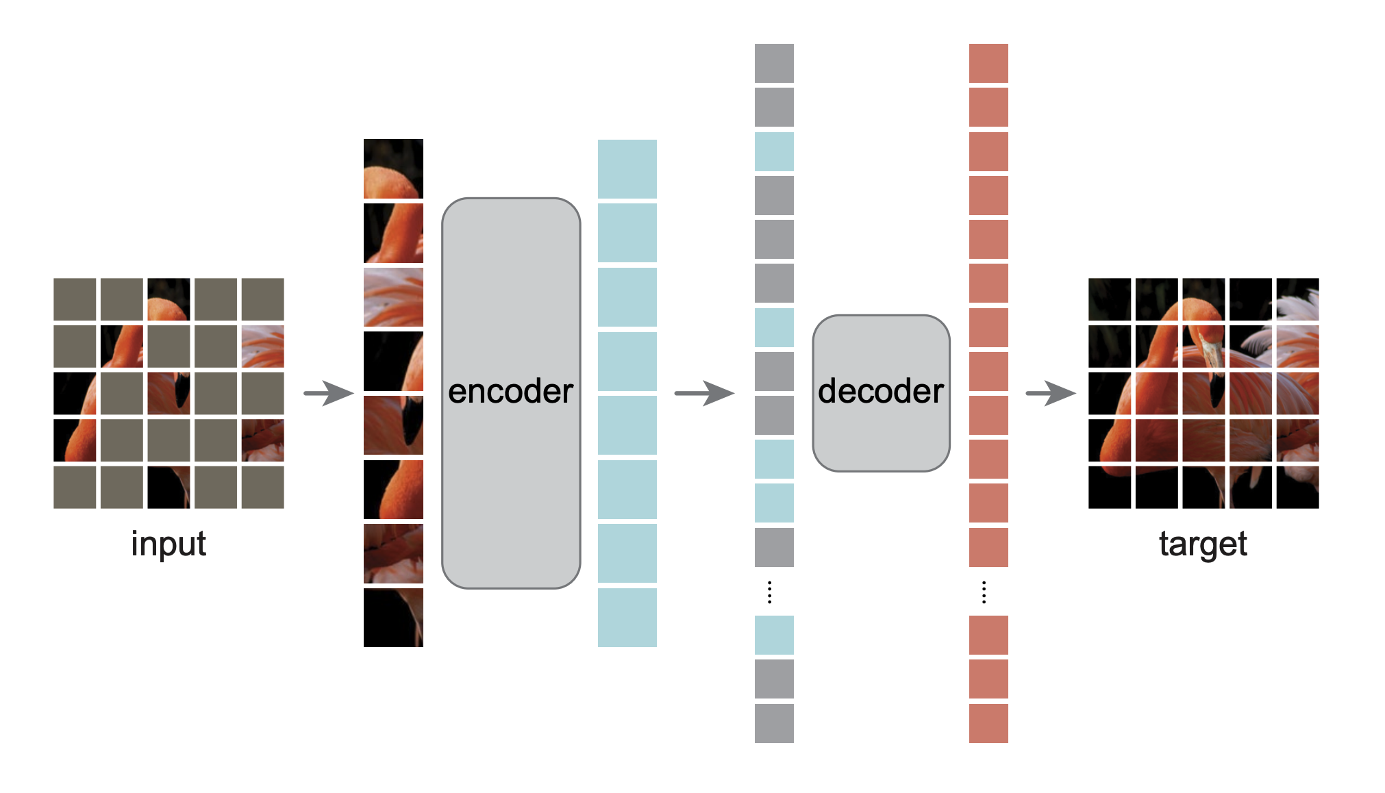
The architecture has two components:

• Encoder (ViT): Processes only the 25% visible patches, learning rich representations from limited information
• Decoder: Reconstructs all patches from the encoded visible patches plus learnable mask tokens

By solving this reconstruction task, the model learns meaningful representations of galaxy morphology (spirals, bars, bulges, mergers) without requiring labels. This learned representation can then be used for downstream classification tasks. Notably, for downstream tasks we really just care about building a strong encoder. In this training setup, because the encoder only processes the visible patches, we can train a much larger encoder than decoder, letting us create a more powerful model for cheaper.

Results

For comparison, I trained a supervised baseline, using the same architecture as the base model. I was able to achieve an accuracy of 68.25%, giving me a good comparison point.

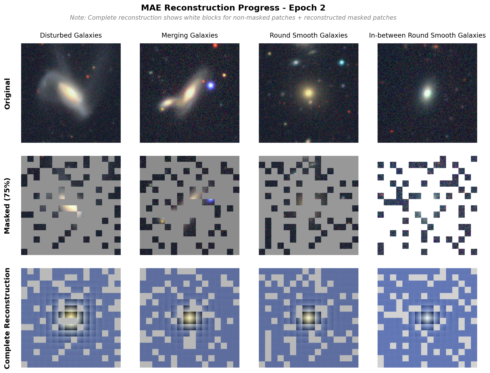
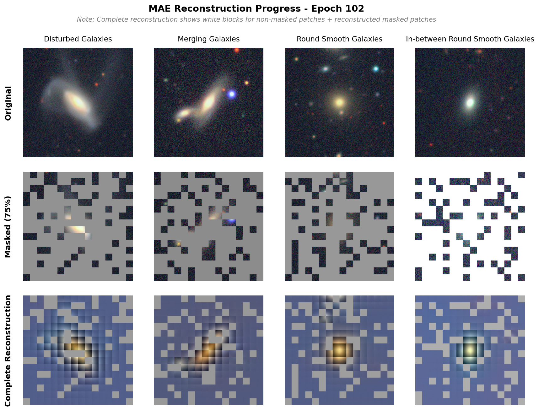
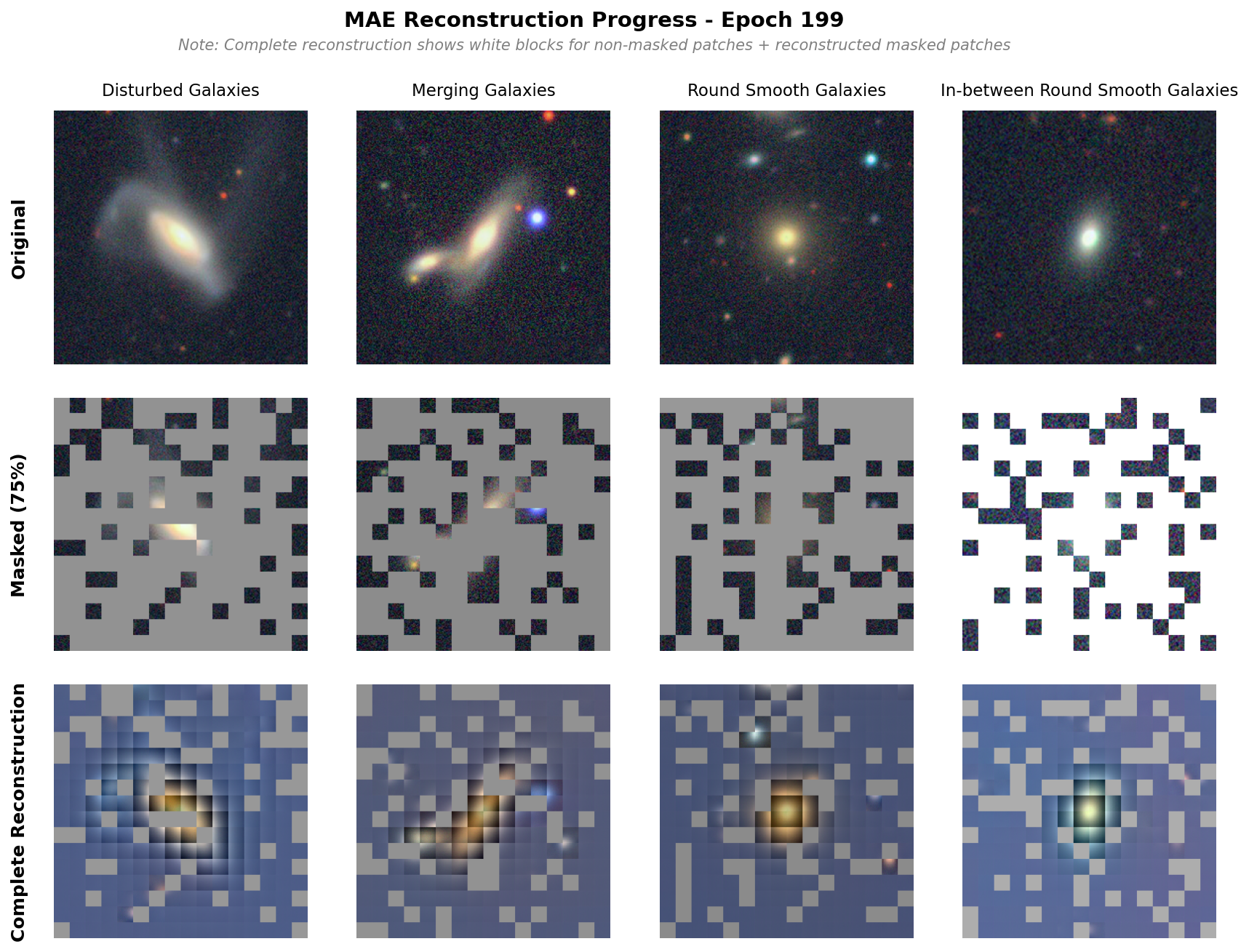
Below is an image of the reconstruction done by the base model. We observe pretty good reconstruction, though there are strong separations between each patch, which is less observed in the original paper. That said, we are able to see the galaxy shapes reconstructed well and subtle features (see the other galaxy in merging galaxy) also appearing.

Model Size

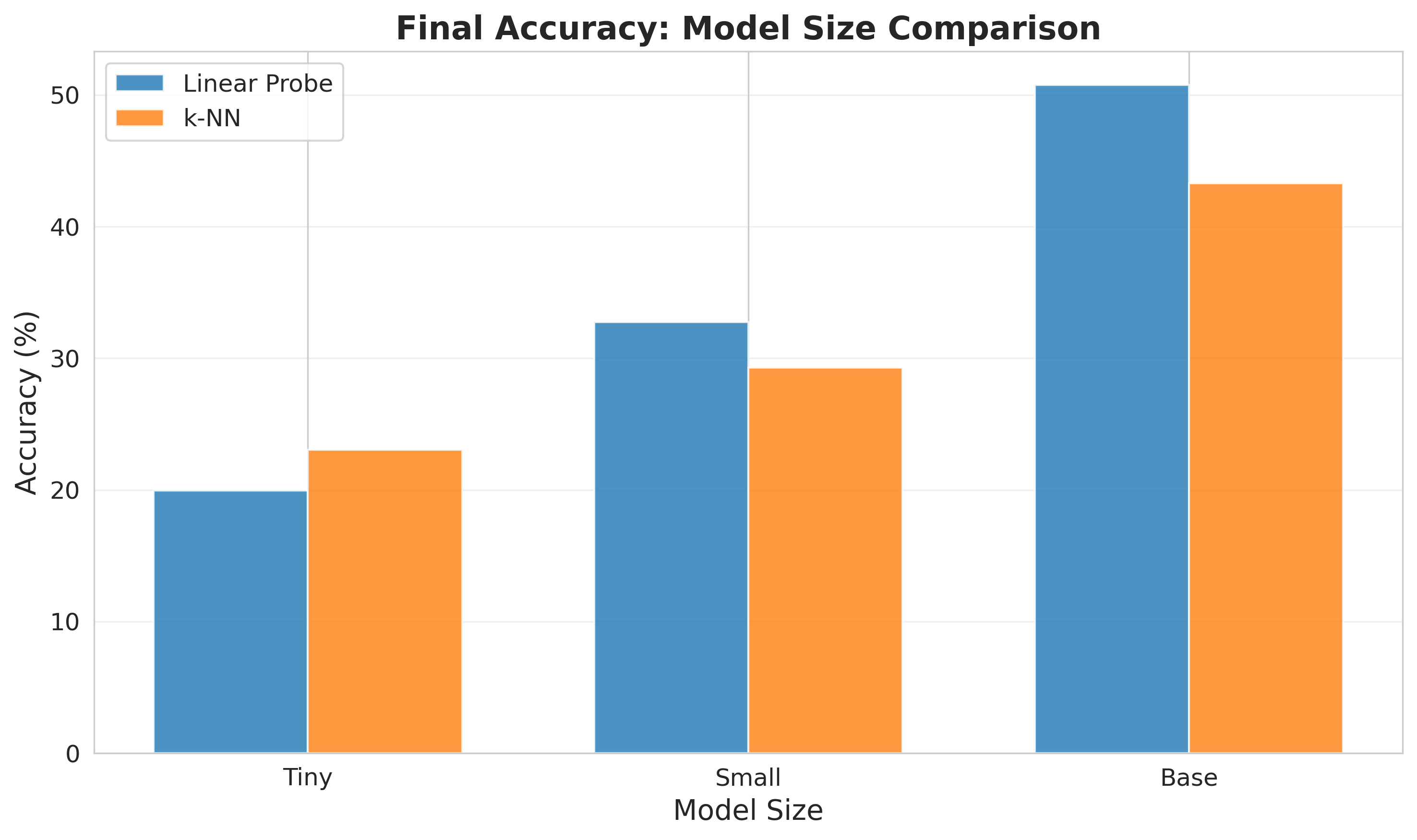
The first comparison I tried was changing the model size. This was also done to test our training pipeline quickly using small models, and is something I plan on doing in the future to give a good reference and confidence as we move to larger training runs. I tried three different sizes: a tiny architecture, a small architecture, and a base architecture. The results are shown below, showing both linear probe and k-NN results from the latent space. We see an increase in performance as the model size increases, and the trend suggests that even larger models would continue to improve performance. Our base model achieves an accuracy of 50.78%.

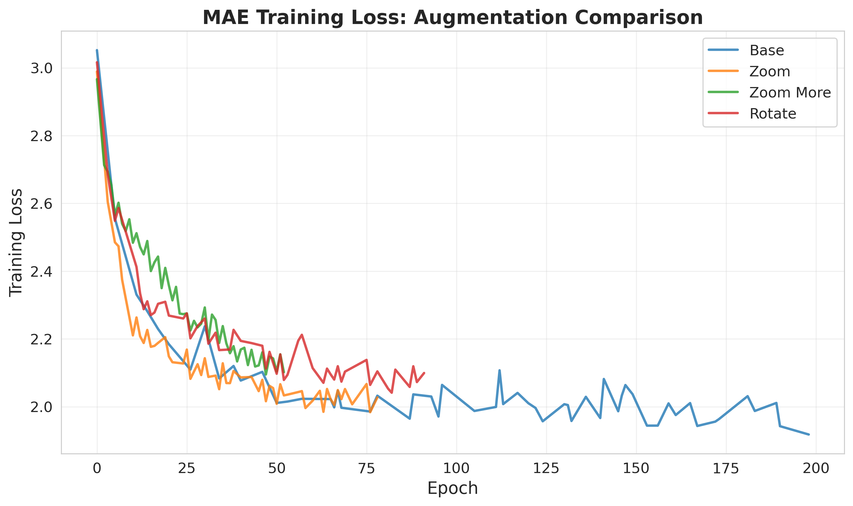
Augmentations

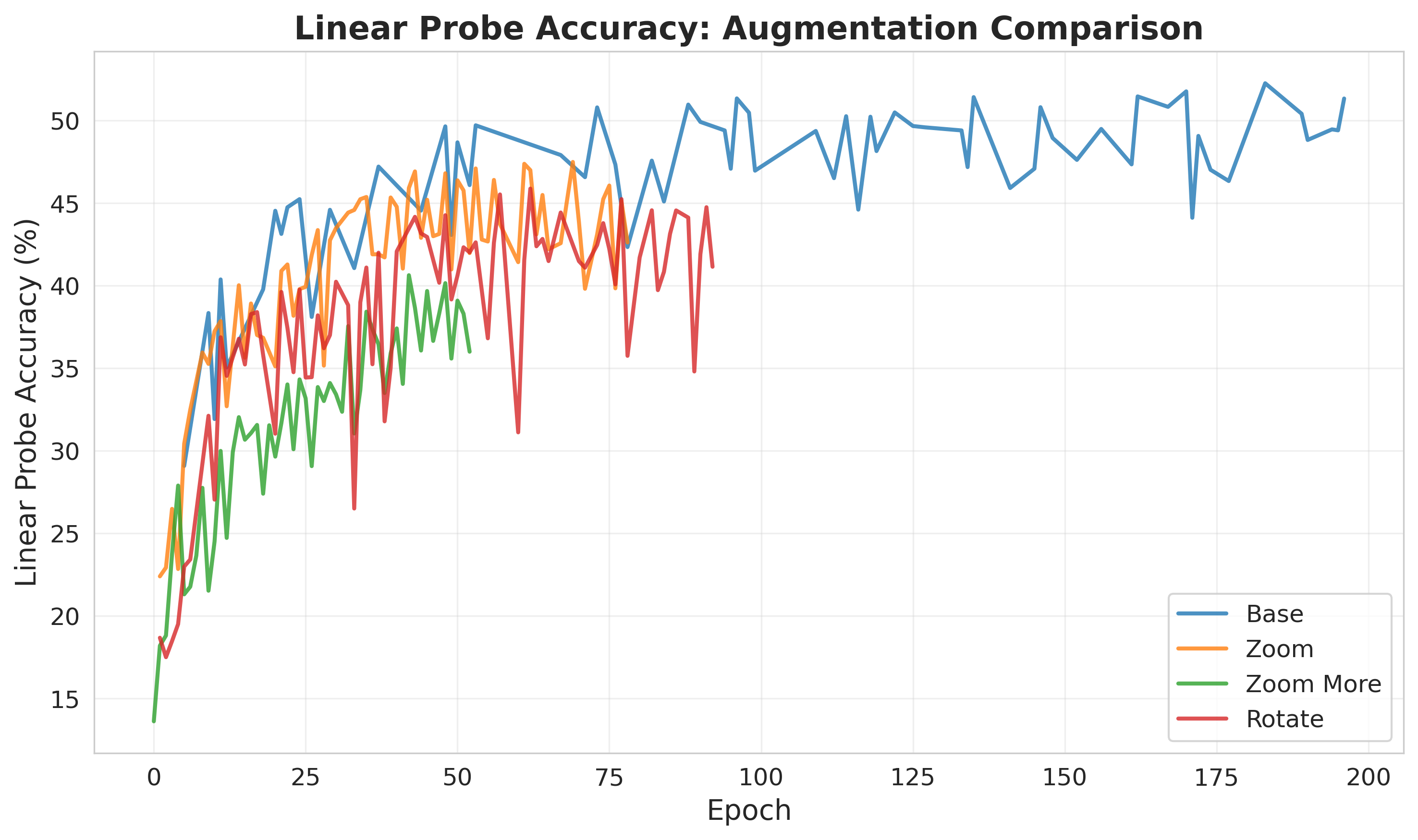
Next, I tried various augmentations. In the MAE paper, they note that the model performs very well without augmentations, but also does slightly better with augmentations. Noticing the galaxies were really just the center of the image, and there was lots of reconstruction wasted on predicting space (basically just noise). The augmentations are applied to the mae task, but the linear probes are trained on the original images. Below are the online linear probe results for the different augmentations. Notably, the augmentations do not improve the performance.

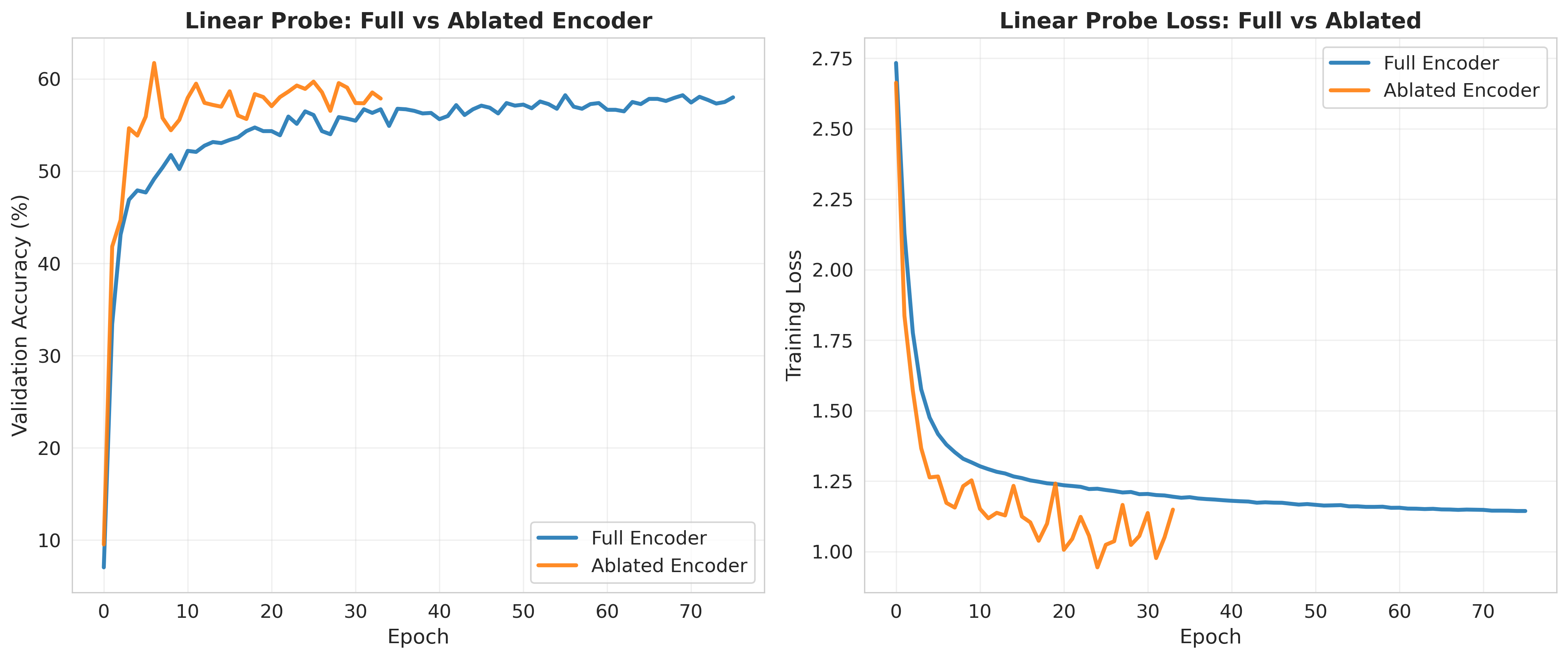
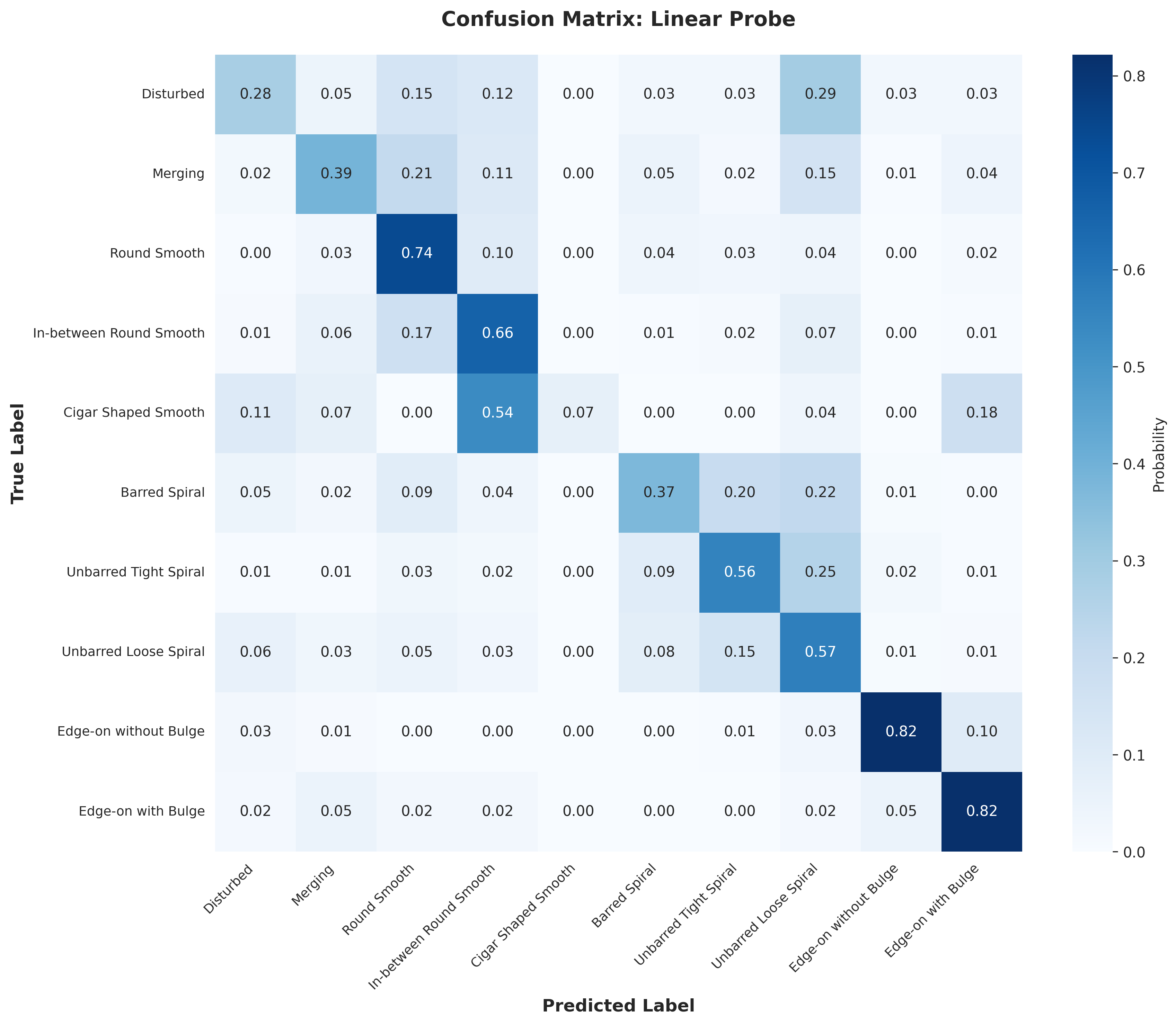
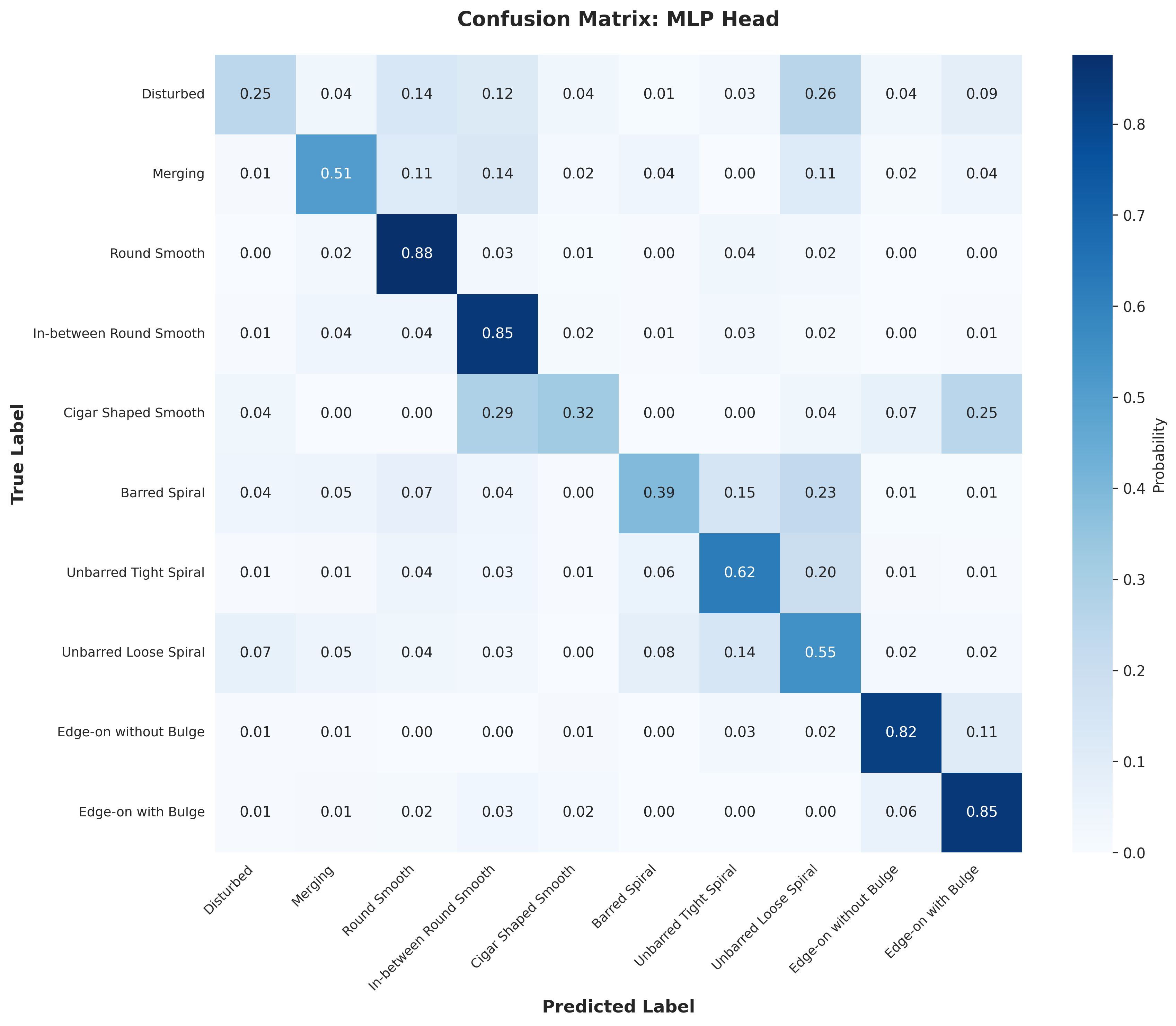
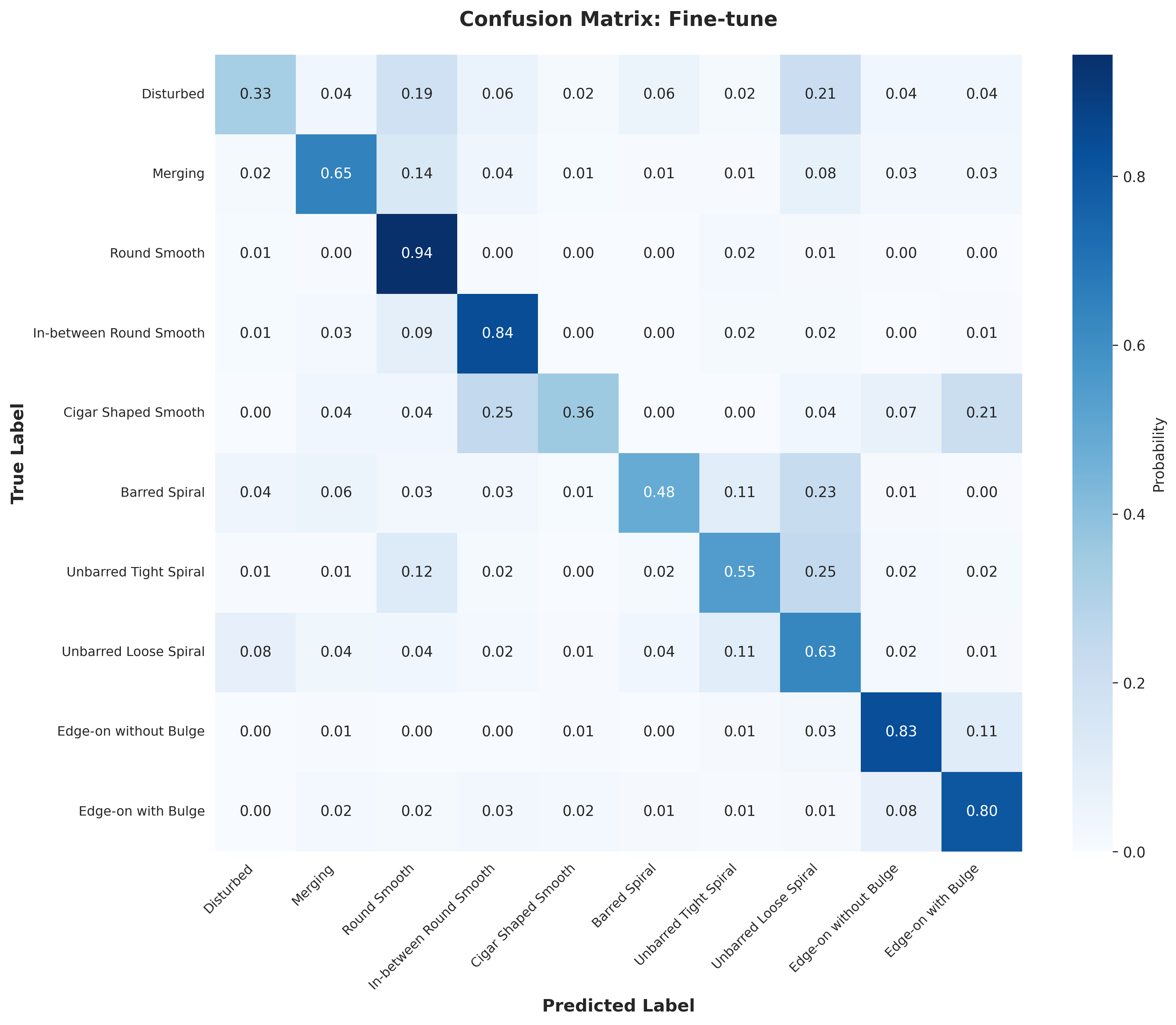
Downstream Architectures

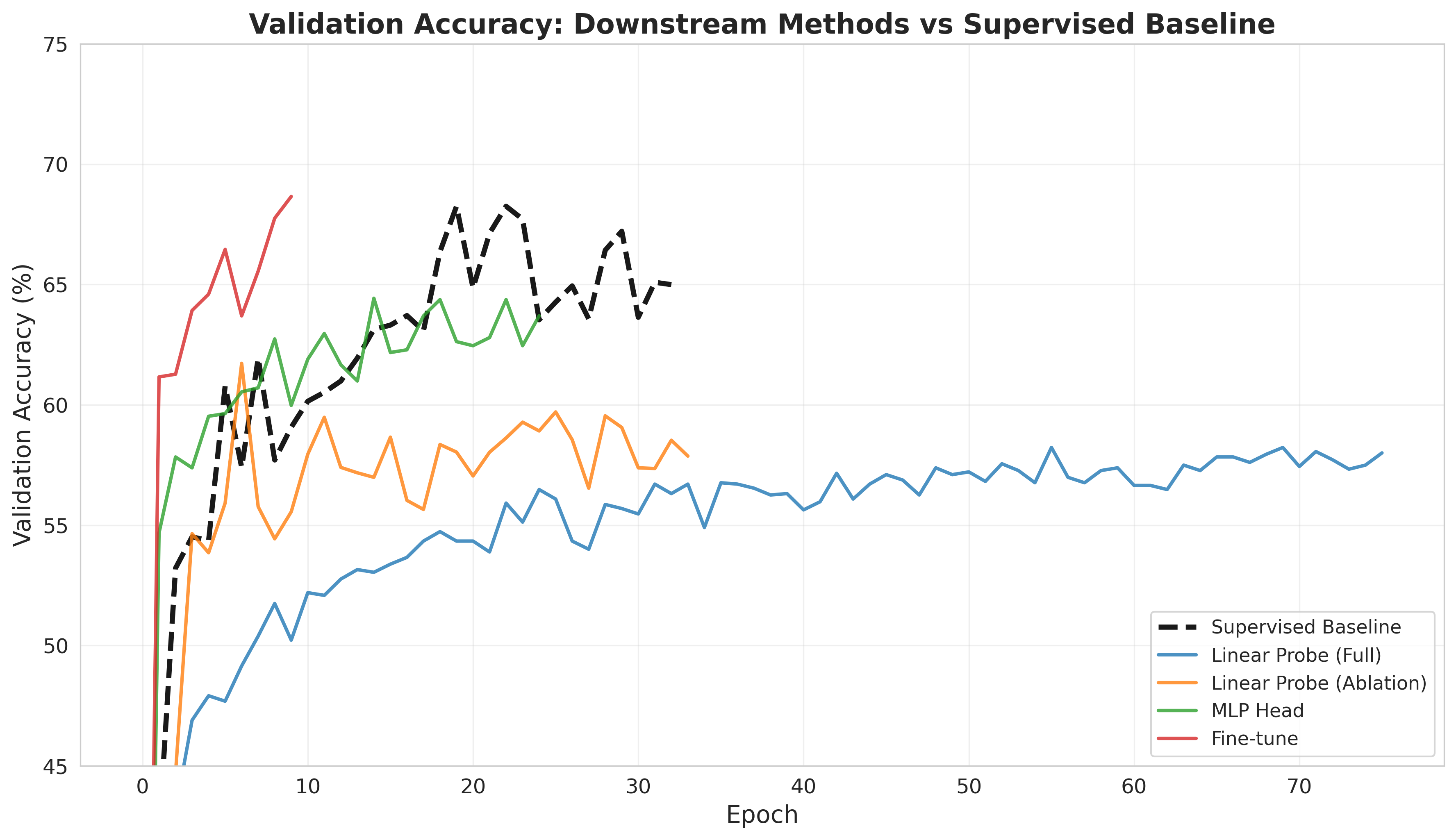
Lastly, using the base model, I tried various downstream architectures to take our latent representation from the encoder and train a classifier. I trained a linear probe on the final output and on the output ablated at depth 8 (out of 12) with the encoder frozen. I also trained a MLP on the final output with the frozen encoder and fine-tuned the model (with a mlp after the final output). Below are the results for the different downstream architectures. They start with the final epoch 199 base model. We see the fine-tuning reaches the same level as the supervised baseline in fewer epochs, the ablated linear probe does better than the nonablated linear probe, and the MLP does better than both linear probes. Overall, I was able to achieve an accuracy of 58% with a linear probe, 63.7% with an MLP, and 67.8% with fine-tuning. The fine-tuning was ended early, and likely would have reached the supervised baseline with more epochs.

Discussion

Overall, the MAE was able to build a decent latent representation. I suspect with more compute we could get better performance. I would be interested in testing other parameters, especially the mask ratio. Nonetheless, our MAE was able to create representations comparable to the supervised baseline using small downstream models.

Weights and biases was a really useful tool for this project, and made it much easier to track and compare my different runs. stable-pretraining was also great for online probing and easy training. Visualizing the reconstruction was also helpful to get a holistic view of the model's performance (and just fun to look at). I also generated some confusion matrices (in the appendix) to get a better sense of the model's performance and found this to be insightful.

Figures