ChessGPT
When I started this project, I set the goal is to build a gpt type model that plays chess, then do interpretability on this to demonstrate various mechanistic interpretability concepts.
I have three phases for this project. At the time of writing this, two of them are completed.
- Pretraining: build and train the model
- Probing: take the pretrained model and learn a linear probe of various points in the residual stream for things like board position, existence of tactics, and more
- Intervention: using the probes, intervene in certain states to adjust the models board state, tendency to predict and act on tactics, and maybe more. It would be great if I could create an interactive model here where I could intervene on the fly and see the effect.
Pretraining
Data
Source
For pretraining and some probing, I am using chess games pulled from the Lichess hugging face dataset. I filter for games in which there are at least 15 moves and both players have an elo of at least 1800. In total, I pull around 40,000 games.
Format
Ad described below, I structure our model to take in the series of moves up to the current state instead of the current board state. On most chess websites, books, and tournaments you will see moves written in Standard Algebraic Notation (SAN). However, most computational chess models use a different format that is part of the Universal Chess Interface (UCI). While the Lichess database is in SAN, we translate this is UCI and use this as input to our model.
Tokenization
UCI moves are structured as [square the piece is moving from][square the piece is moving to]<promotion>. Castles can be represented in this format as moving the king to the location after castle.
Task
Chess is, aside from modeling player behavior, Markovian. When deciding on a move, what matters is the current position not the sequence of moves that led there. This means the strongest formulation of a chess prediction task would take the current board state as input and predict the best move, essentially learning a value function over positions.
But that's not the formulation I chose. My goal is to learn about mechanistic interpretability through models that resemble large language models. To mimic the self-supervised next-token prediction paradigm of LLMs, I instead frame the task as sequence prediction: given the moves played so far, predict the next move.
Formally, given a sequence of moves , the model learns a function that takes and predicts . Just as language models can extract training examples from a single sentence of length (by masking increasingly longer prefixes), I extract training examples from each chess game.
This formulation has an interesting implication: the model must implicitly reconstruct the board state from the move sequence. It cannot simply "look" at the current position. Instead, it must track how each move transforms the board. This makes the internal representations potentially richer and more interpretable.
Model
The architecture is a GPT-style transformer based on NanoGPT. The pipeline consists of:
- Tokenizer: Converts UCI move notation (e.g., e2e4, g1f3) into token IDs
- Embedding layer: Maps tokens to dense vectors and adds positional encodings
- Transformer blocks: 12 layers, each containing: a) Multi-head self-attention b) Feed-forward MLP c) Layer normalization and residual connections
- Output head: Projects the final hidden state to a probability distribution over all possible tokens
In total, it is only 88.M parameters. The model outputs a probability distribution across all moves in the vocabulary. During inference, the predicted move is simply the one with the highest probability.
The model was trained using cross-entropy loss, comparing the predicted probability distribution against the actual next move played in each game.
Evaluation
Predicting the exact move a human played is a noisy target, as multiple moves might be equally good in any position, and playing styles vary widely. So I evaluate the model along several dimensions. I was also interested in how these metrics change with respect to the move number in the game. Below are the metrics I evaluated.
Accuracy
What percentage of predicted moves match the moves actually played? This is a strict metric: even if the model's prediction is an excellent move, it counts as wrong if it differs from the game record.
Legality
Perhaps more fundamental than accuracy: is the model even making legal moves? For any board position, the vast majority of possible UCI strings represent illegal moves. There are at most 20 possible starting squares for a side's pieces, and each piece has limited legal destinations depending on its type and the board state. I measure legality two ways:
- Top-1 legality: How often is the highest-probability move legal?
- Legal probability mass: What fraction of the total probability distribution is assigned to legal moves?
Confidence
How certain is the model in its predictions? A maximally confident model would assign 100% probability to a single move. A minimally confident model would output a uniform distribution. I quantify this using entropy:
Lower entropy means higher confidence.
Results
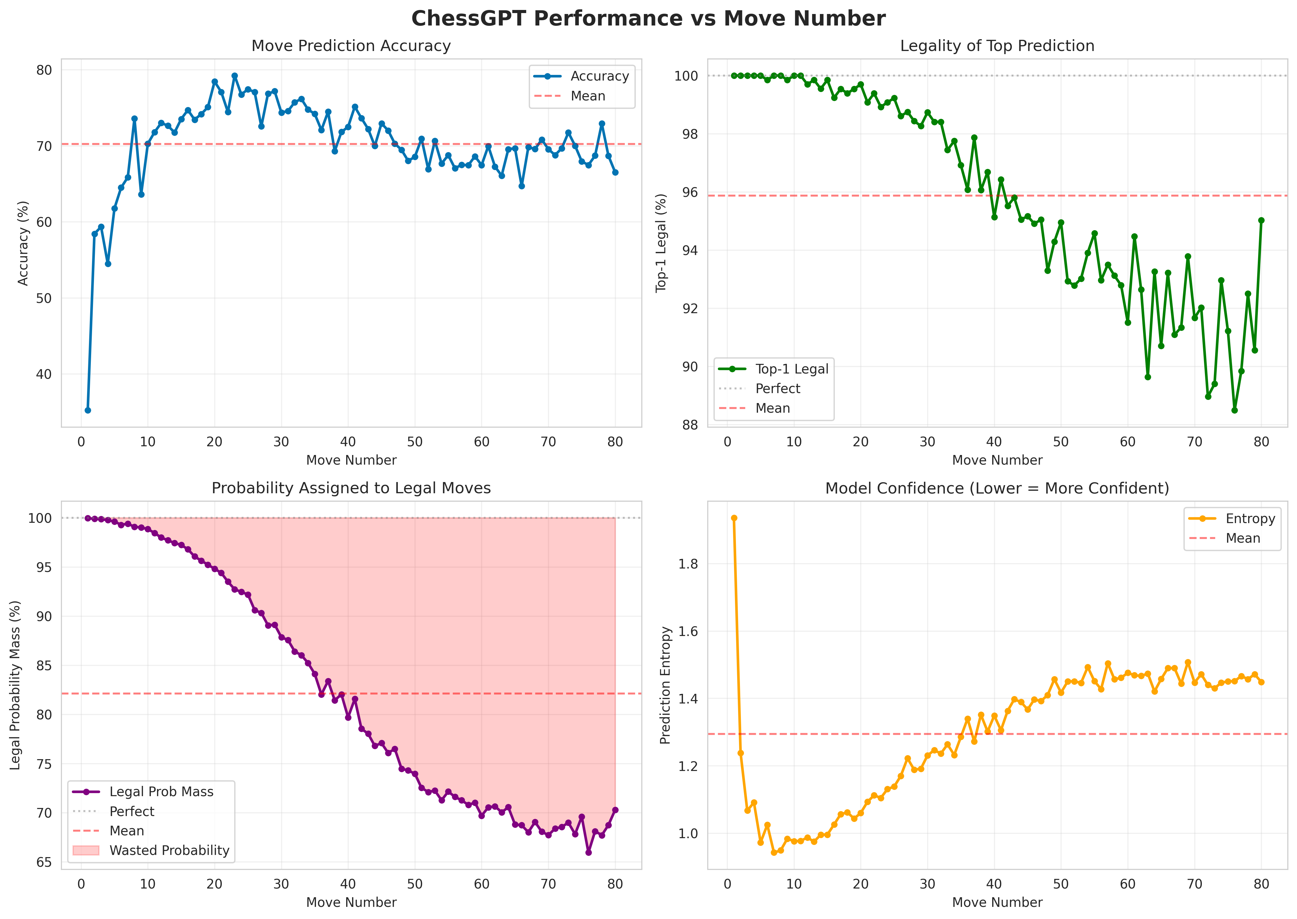
For all the graphs, note the scales. We see decent accuracy, with rather low accuracy in the opening, highest accuracy during the middlegame, and a plateauing as it reaches the end game. We see very good performance for legality. Notably, where the accuracy is low at the start the the game, the legality is perfect. This makes sense, as there are many openings and it is an ill-posed task to predict what opening someone is going to play. But as the game progresses, the number of good moves to make in a position becomes a much smaller set. In both Top-1 and probability mass, we see a sigmoid-shaped curve with decreasing performance for later moves, but still strong performance overall. Lastly, in terms of confidence, we see validation for the opening, in which the model has very low confidence in its predictions, with entropy decreasing rapidly. Then, as the game progresses, the entropy increases and the model becomes less sure of which move to make.
As an exercise, here's ChessGPT's response to 1. e4, the most common opening move:
| Rank | Move | Probability |
|---|---|---|
| 1 | c7c5 | 25.44% |
| 2 | e7e5 | 24.15% |
| 3 | e7e6 | 17.53% |
| 4 | c7c6 | 9.02% |
| 5 | d7d5 | 6.19% |
| 6 | d7d6 | 5.23% |
| 7 | b7b6 | 3.99% |
| 8 | b8c6 | 3.56% |
| 9 | g7g6 | 2.39% |
| 10 | g8f6 | 1.82% |
Top 10 predicted responses to 1. e4
These are all legitimate, commonly-played responses to 1. e4, ordered roughly by popularity in real games. The model has learned the statistical distribution of chess openings.
Then, I played a few games with it. Anecdotally, while it is far from a great chess player, it is not an awful player. It handles openings reasonably well, makes sensible developing moves, and occasionally finds nice tactical ideas like forks. But it also misses obvious opportunities like a free piece sitting in front of a pawn, or an escape via check when under attack.
It plays like someone who has just learned the rules and understands how pieces move, but hasn't yet developed the pattern recognition that makes strong players. This is perhaps unsurprising: the model was trained to predict human moves, not to win games. It has learned the distribution of chess, not the optimization of chess.
Probing
While the model is able to perform well, I would like to know what is actually going on. What is the model learning? How is it able to know which moves are legal? To do this, I make use of probes, specifically linear probes. There is an idea called the Linear Representation Hypothesis which proposes that high-level concepts are encoded as simple, straight directions in LLMs' representation space. It has been shown that a similar model trained on Othello learns a linear representation of the board. My goal is to linearly probe for various concepts and help determine what the model is learning.
Setup
With a frozen, pretrained model, we pass a data point through, then grab the latent values (aka residual stream) between every layer. We could even go as far as sampling between attention and mlp layers to understand the affects of each, but I treat these as one unit and sample between attention-mlp pairs. Additionally, it may be insightful to train a different probe for even and odd moves, but for simplicity (and compute) I opt to train one probe per layer per concept across all moves.
For each data point we pass through, we know some ground truth that is not immediately obvious upon looking at a sequence of moves. For example, an easy property is whose move it is: black or white. We construct a dataset across many games which consists of the moves as input and the ground truth property as the label. Then, we run the model and train a linear probe on each layer that takes in the residual stream at that layer and predicts the ground truth property.
The properties I decided to test were:
- Turn. A binary classifier that predicts whose turn it is. The simplest probe, and because of the high legal move rate, I expect very good performance on this.
- Square Occupancy. For each of the 64 squares, I train a separate probe that predicts if that square is occupied. This is a simplified board state probe.
- Piece Location. Here, I ask where each piece is located. For all 12 piece types (6 white and 6 black), an independent multi-label binary classifier predicts a 64-dimensional binary vector that indicates which squares that piece occupies.
- Material. There are two probe types here. First, I have 12 probes, one for each piece, that predict the count of that piece. Then, I have one probe that predicts the material balance (in pawn units). These are all ridge regressors. I am unsure on performance here, as material balance is not necessarily the best representation of the game.
- Positional Rules. These probes test hidden game state features not visible on the board. There are five binary classifiers for white can castle kingside, white can castle queenside, black can castle kingside, black can castle queenside, and en passant available.
- Board State. In addition to the square and piece probes, I wanted a granular board state reconstruction system. I train one binary classifier for each piece for each square, giving 832 () probes per layer. In hindsight, this may have been overkill and took a long time to train, but it is definitely comprehensive and gives us a nice peak into the model's view of the board.
- Tactical. For a series of tactical puzzle themes (fork, pin, skewer, etc), I train a classifier. For this, I used puzzles from the Lichess puzzle dataset. Each datapoint has a set of theme associated with it, giving us some ground truth, even if the length of the puzzles differ. This dataset is positional, meaning it doesn't have the moves, so I grabbed the gameID from each puzzle and used the Lichess API to get the moves from each game up to the puzzle start. Also, while other concepts here were important for playing legal moves, this is not necessarily true here, and tactics are quite high level, so these results will be interesting.
Probing Results
Turn Probe
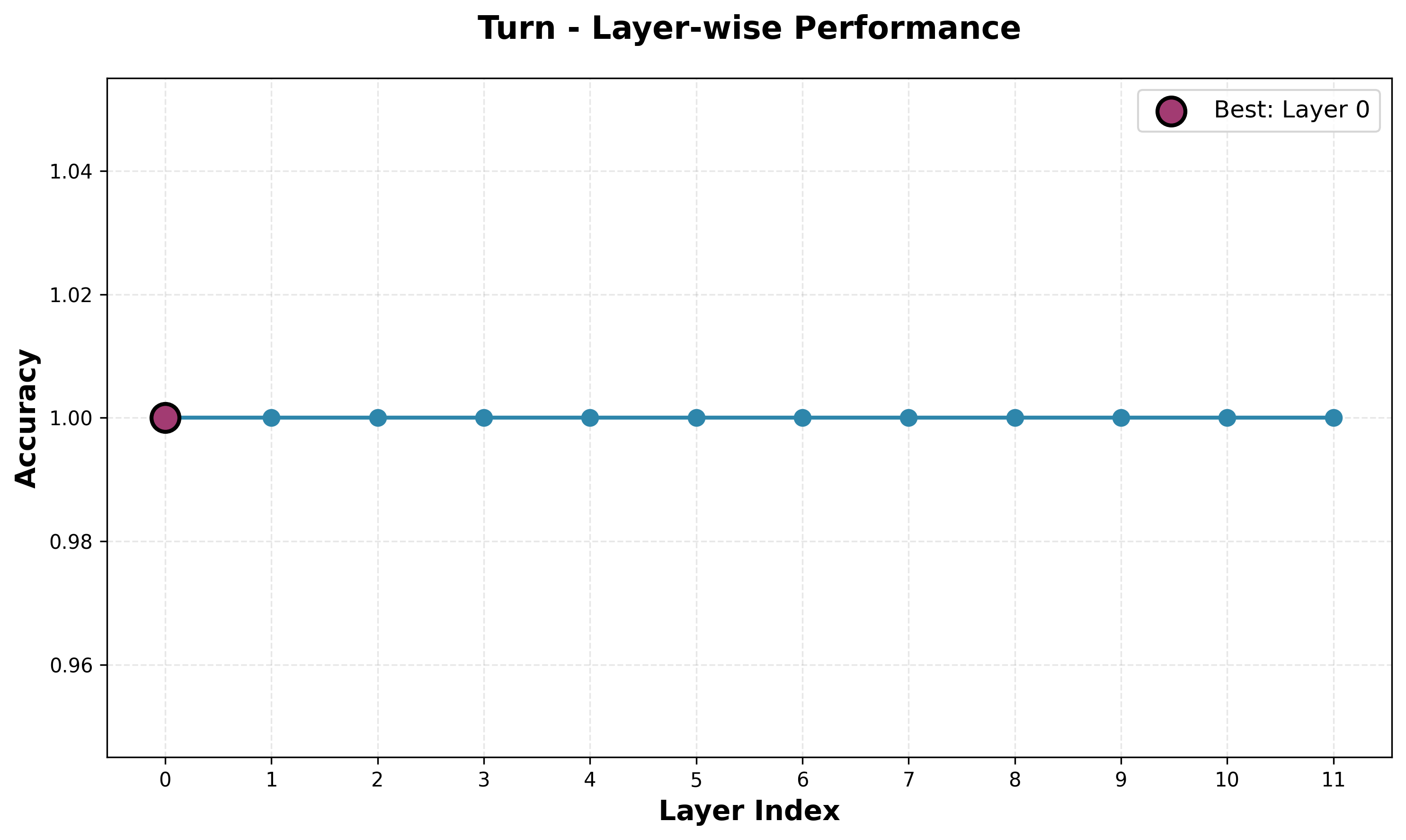
To no surprise, the turn probe has perfect accuracy across all layers. Given the model's ability to predict legal moves, it must know whose turn it is, and pretty much any decisions about what the next move is going to be depend on who is moving. It would be interesting to see how the model is predicting this, as it could be taking some modulo of the number of moves so far, memorizing that even moves and odd moves correspond to black and white (one indexed), or even using the previous move to deduce who just moved.
Square Occupancy Probe
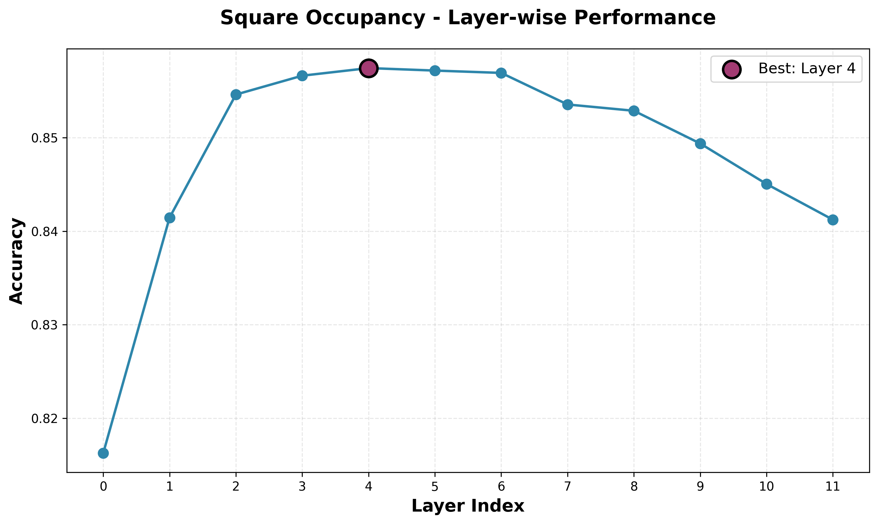
We see strongest square occupancy performance from layer four, with decent, but far from perfect accuracy. Interestingly, the accuracy is lower for the first few layers, before peaking at layer four then steadily dropping. We expected to see lower-level concepts have stronger representations in earlier layers and high-level concepts represented in later layers. Quantifying the "high-levelness" of a concept is a far from exact science, but we can take a rough, intuitive guess for each of our concepts. For turn, this is obviously very low-level. For square occupancy, this is not extremely low-level, but still relatively simple compared to the concepts required to play chess.
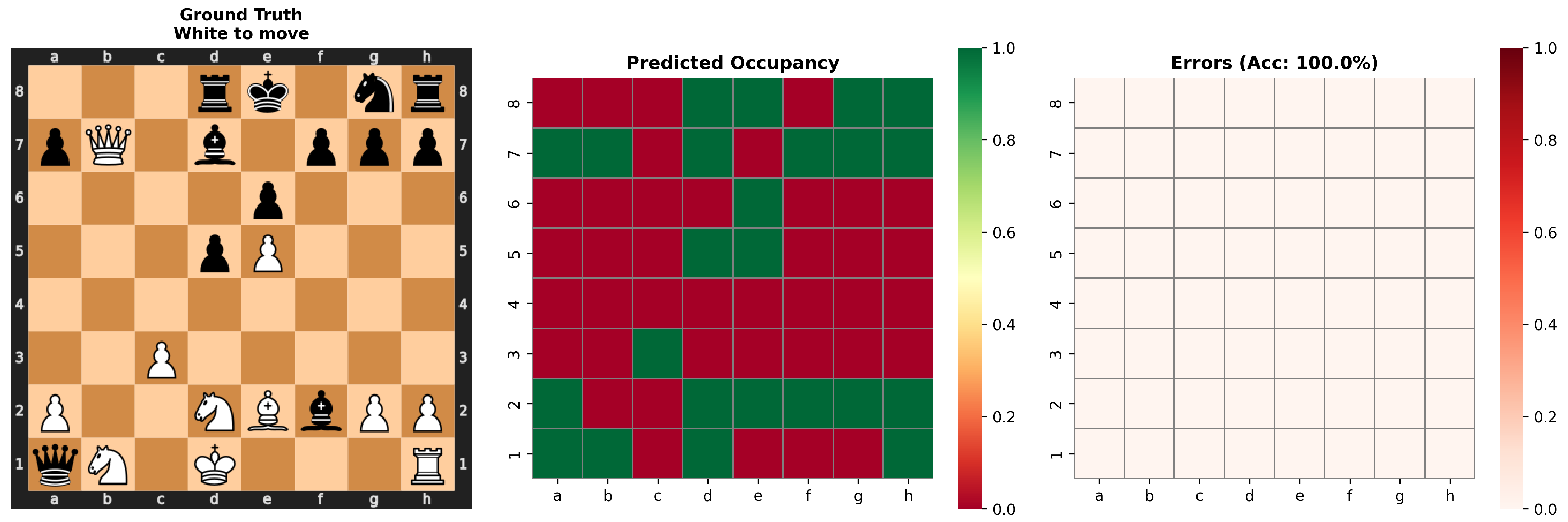
Examining some specific cases when probing layer 4, we see the model has a strong understanding of square occupancy even in complicated cases. In one position, the opening looks standard, except white's king is moved from its home on e1 to f1. The model misses this, thinking e1 is occupied and f1 is open. This suggests that while the model is strong in common positions, it breaks down in strange positions. This poor out-of-sample performance was an original issue with AlphaGo, and is attributed to its loss in the 4th game against Lee Sedol.
Piece Location Probe
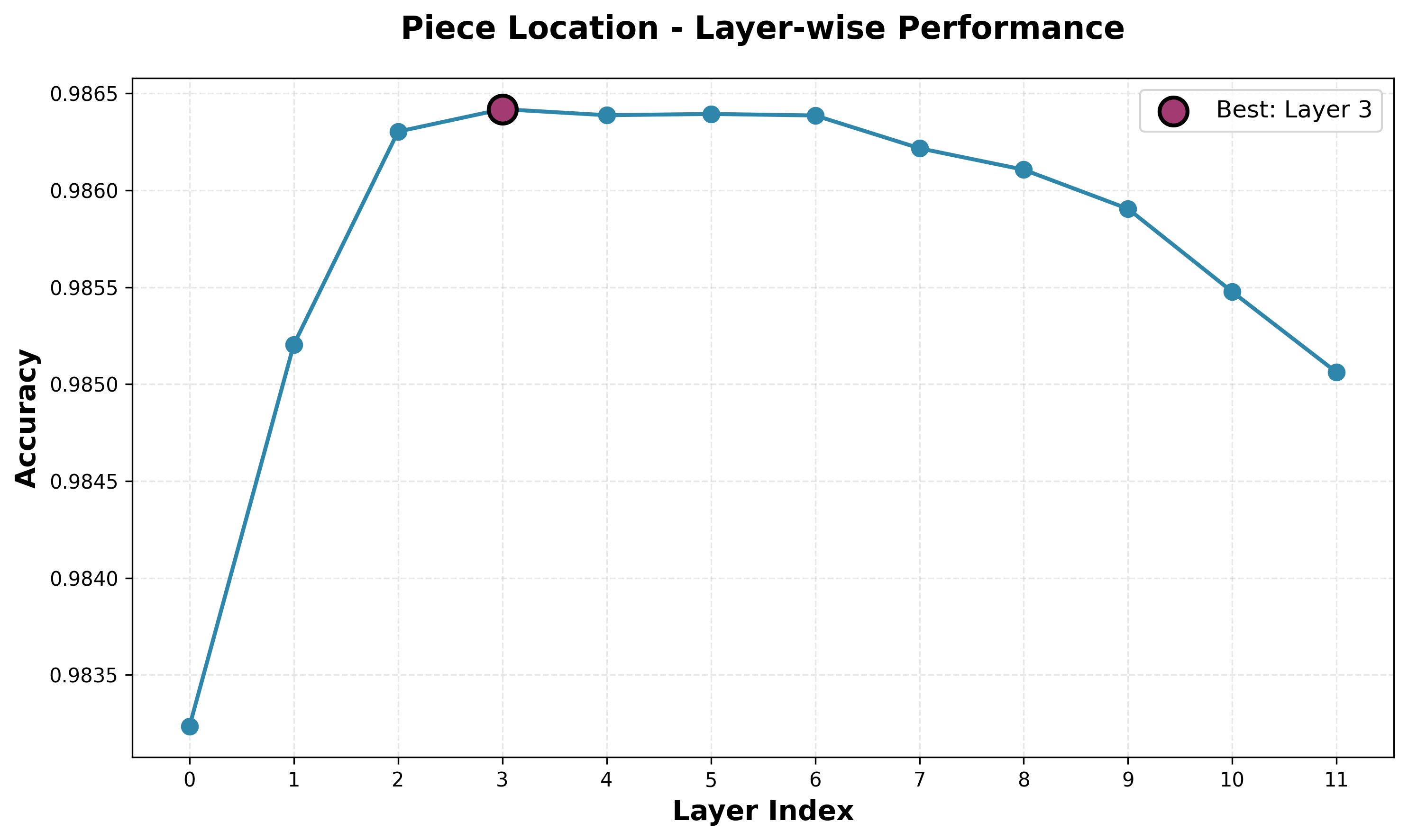
Our piece location probe has incredibly high accuracy. Note accuracy scale: the difference between the best and worst performing layers is only 0.003. Still, despite the scale we see a clear pattern emerge, with best performance at the early middle layers and a slowly decreasing performance with later layers. It is an almost identical curve to the square occupancy curve. The high performance suggests the piece location is very important to the model, which makes sense. The performance over the simpler square occupancy tasks also suggests that the model is storing information in a manner similar to this task. Sensibly, piece-level information is much more useful than square occupancy.
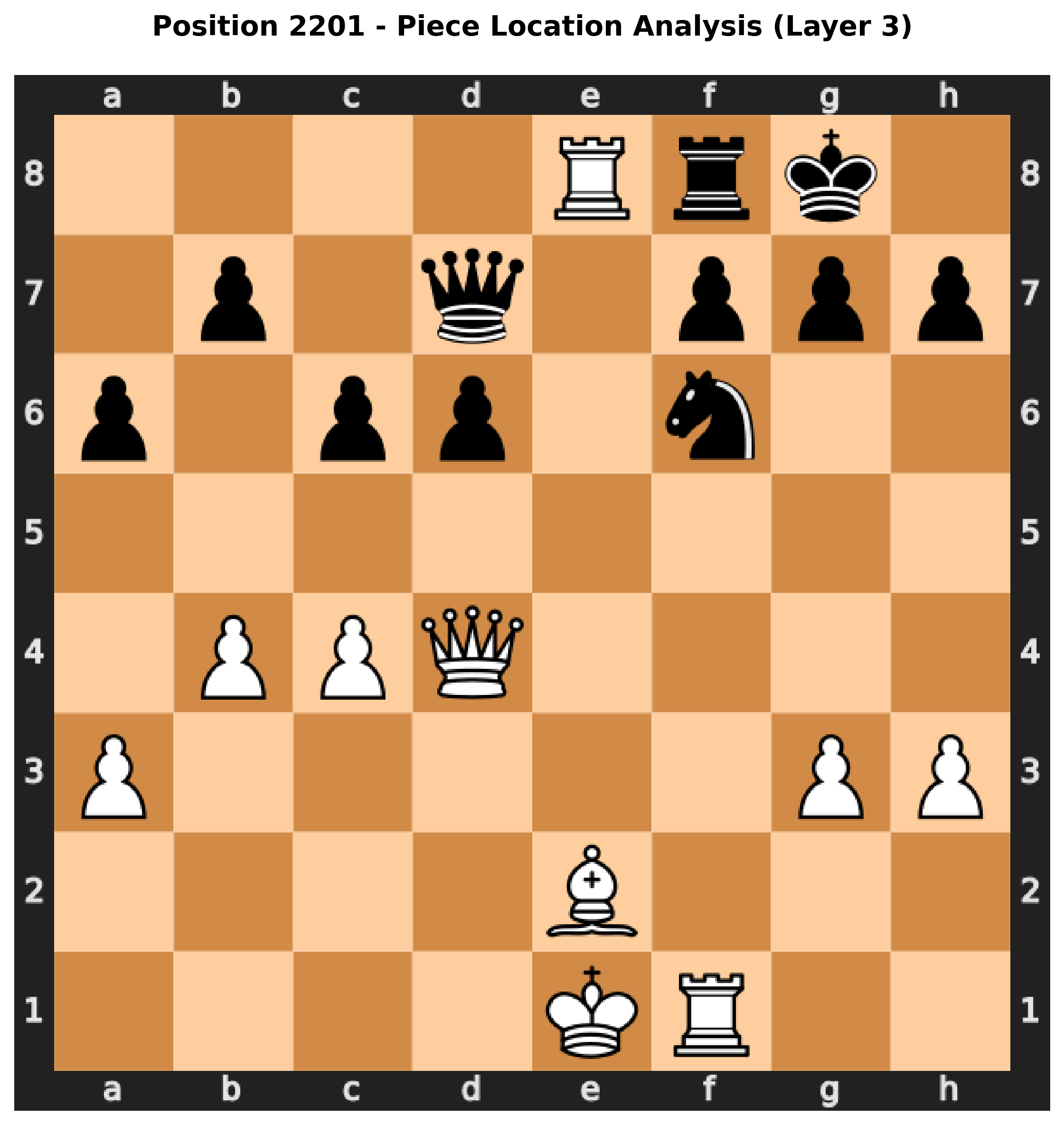
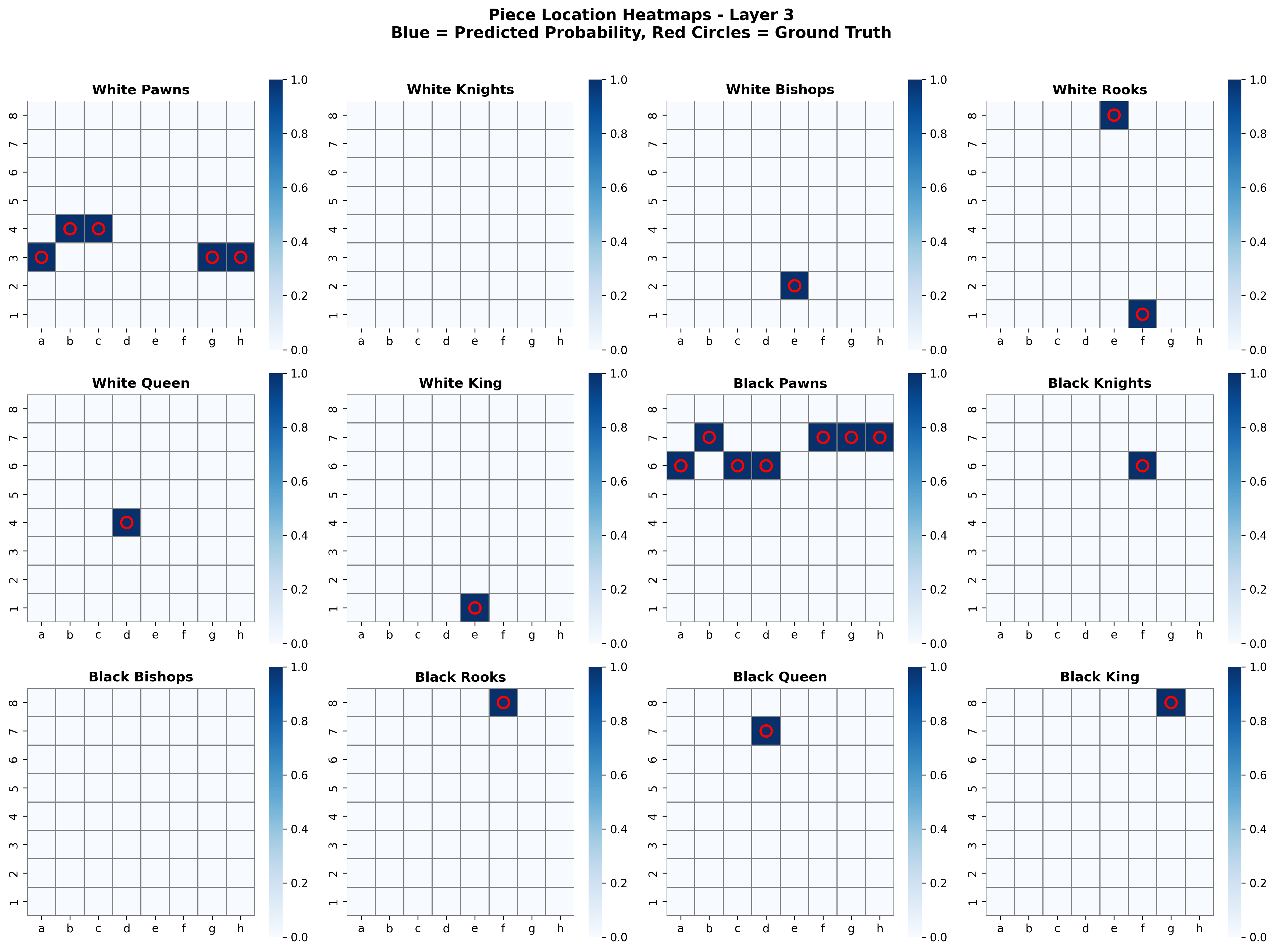
Here we see the predictions of the piece locator probes for a random position. While this position is not complicated, it is not simple, but the model is able to predict the exact locations for each piece type, including predicting the right number of pawns, only one location for pairs that have lost a piece, and no locations for piece types completely captured.
Material Probe
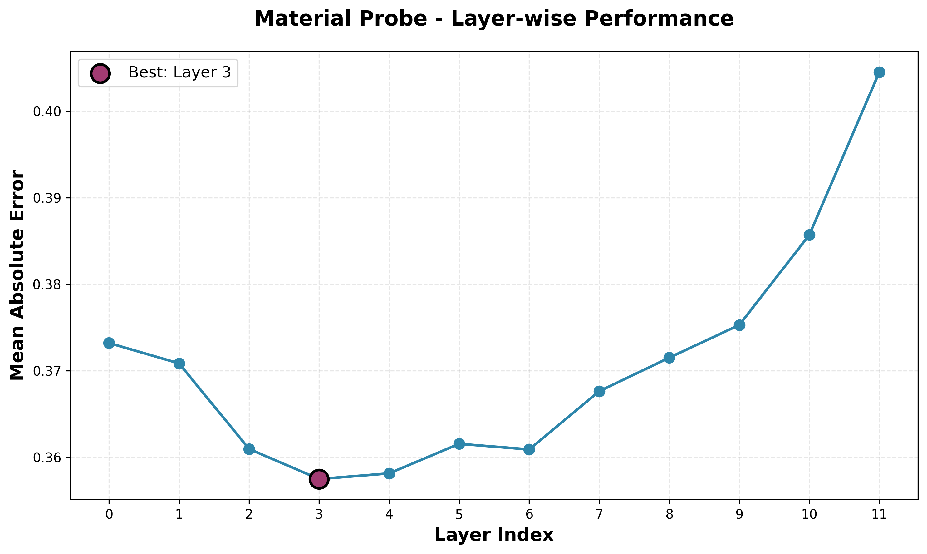
Here, I am graphing the mean absolute error (MAE) in predicted material difference and actual material difference, so lower is better. We again see the same trend as the piece location and square occupancy curves, which makes sense, as the material difference is simplified version of the piece location task. The MAE is also quite low, which is sound given the accuracy of the piece prediction probe.
Positional Rules Probe
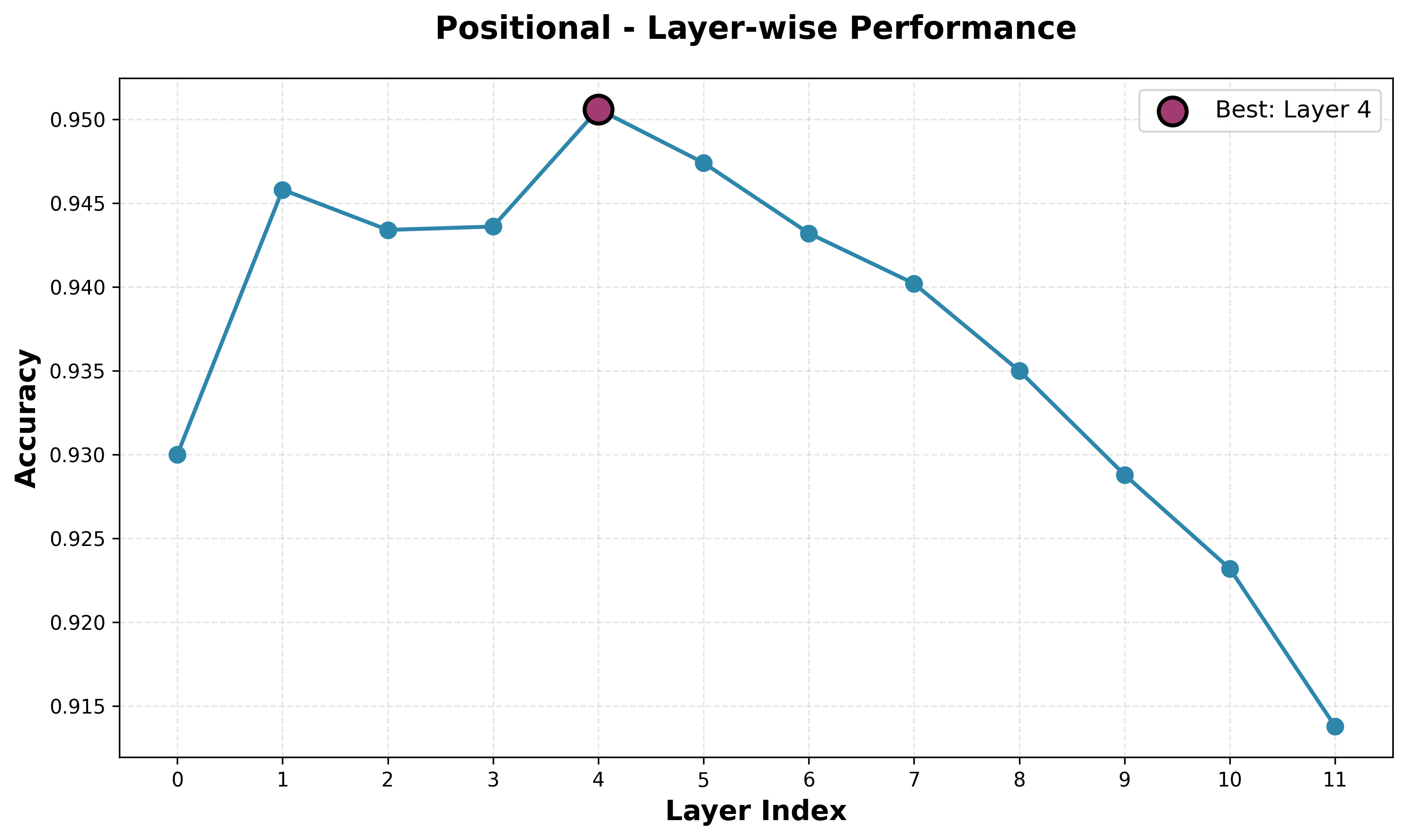
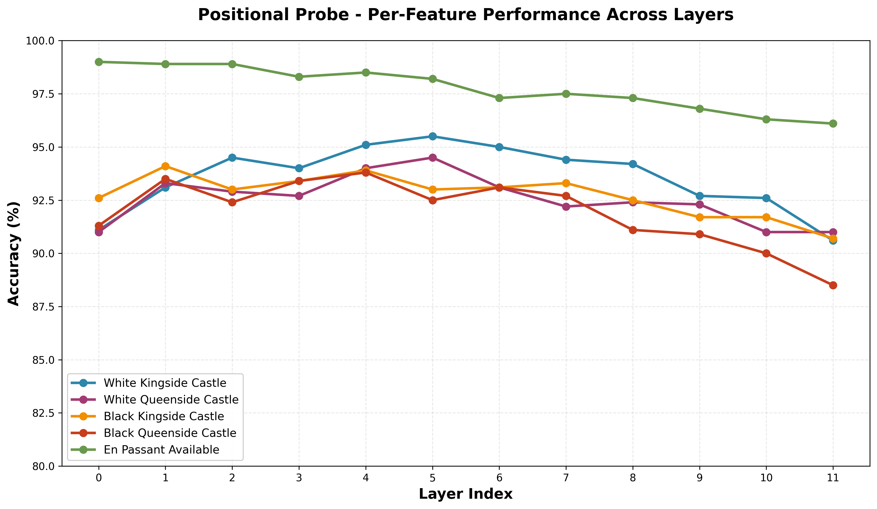
The model has decent understanding of hidden positional rules. While the average performance peaks in layer 4, we see this is not necessarily the best layer for each of the individual features. En Passant has a near monotonic decrease in performance after layer 0. The castle performances are all similar, though comparing side performances (kingside vs queenside) for white and black, we see a constant stronger performance for white, and within white and black we see a constant better performance for kingside over queenside.
Board State Probe
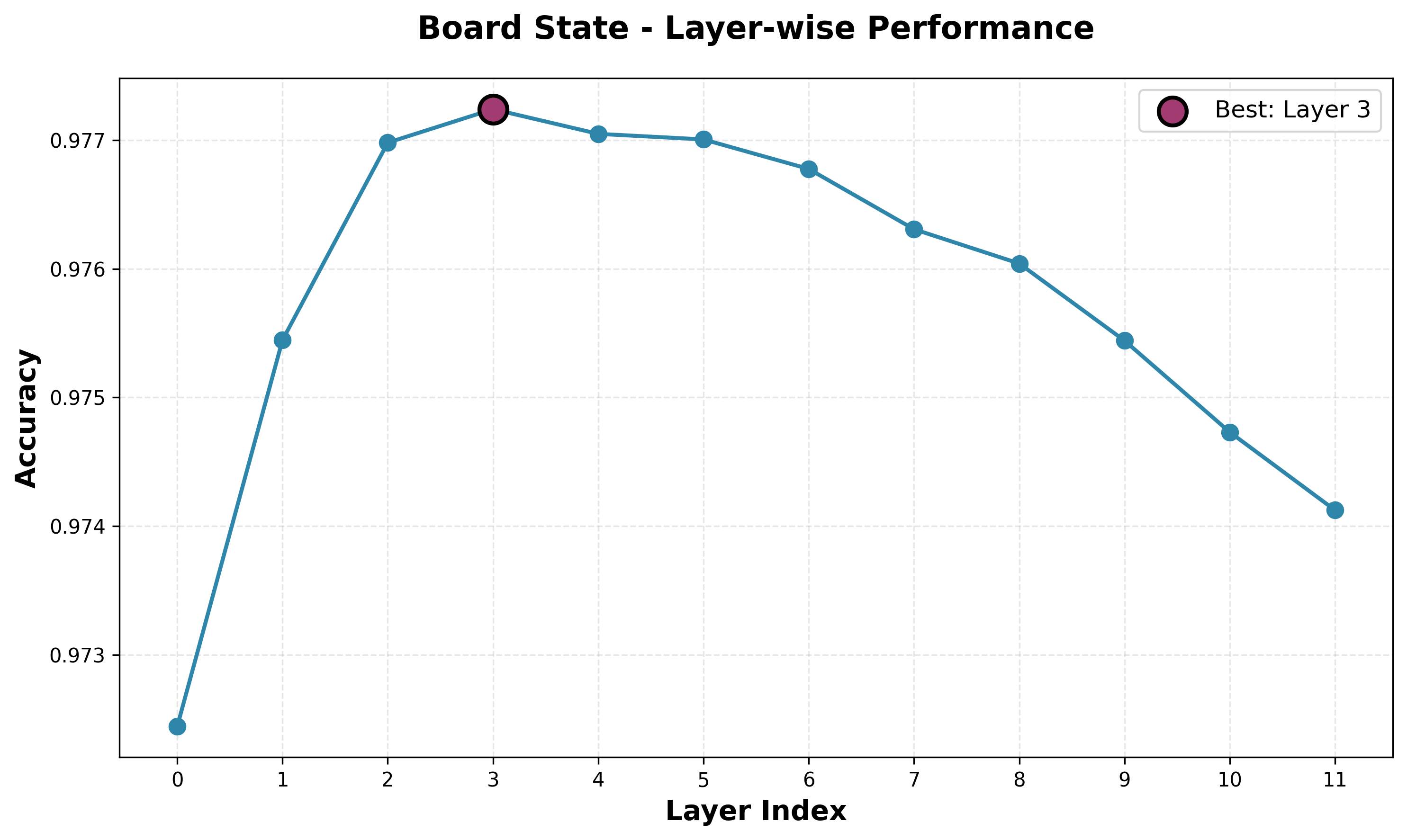
The board state probe shows the same shape and similar performance to the piece position probe. This is just another way of trying to capture the same state, so it is validating to see that they both have similar performance.
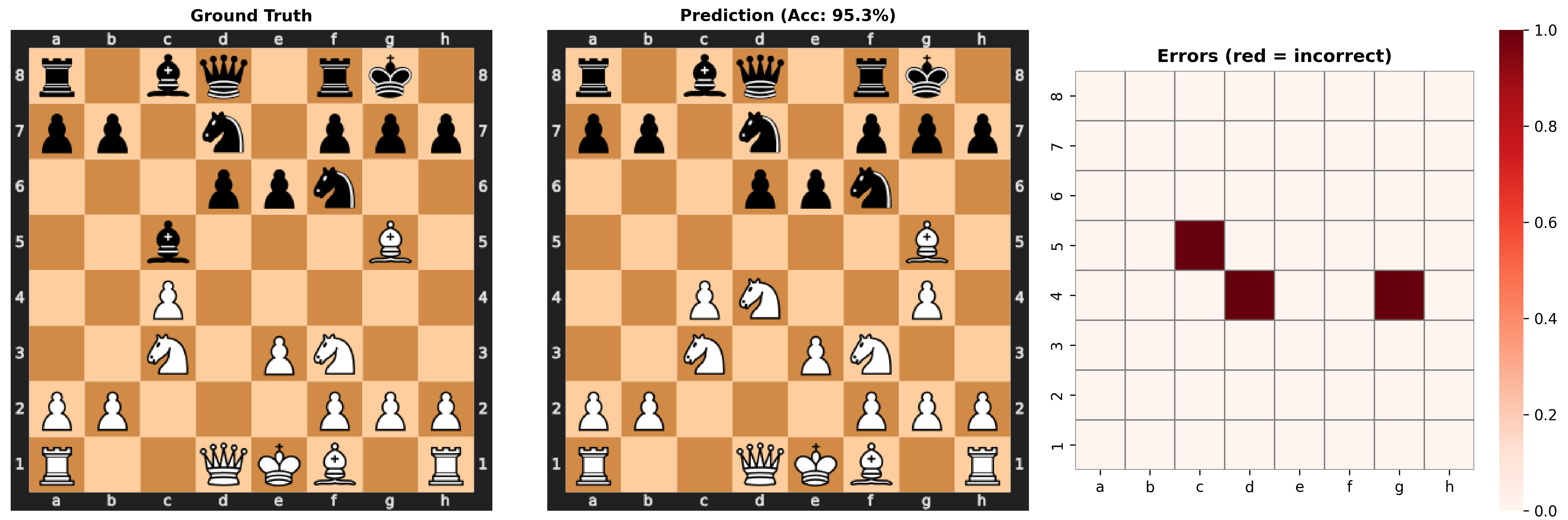
Looking at some random positions, we can see that most of the time it does a perfect job reconstructing the position. Occasionally, it will make small errors, some of which are nonsensical like three knights. Sometimes, however, it fails a lot of the pieces, even though it still gets a decent accuracy. It seems in these catastrophic failures, it fails in nearly every way: it misses some pieces, it moves some pieces, and it replaces a bunch of pieces with pawns, including white pawns on the eight rank and the first rank! This suggests that in these cases it is not just one probe or one small part of the representation that is insufficient, but a large part of the representation that contains the information about many locations and pieces.
Tactical Probe
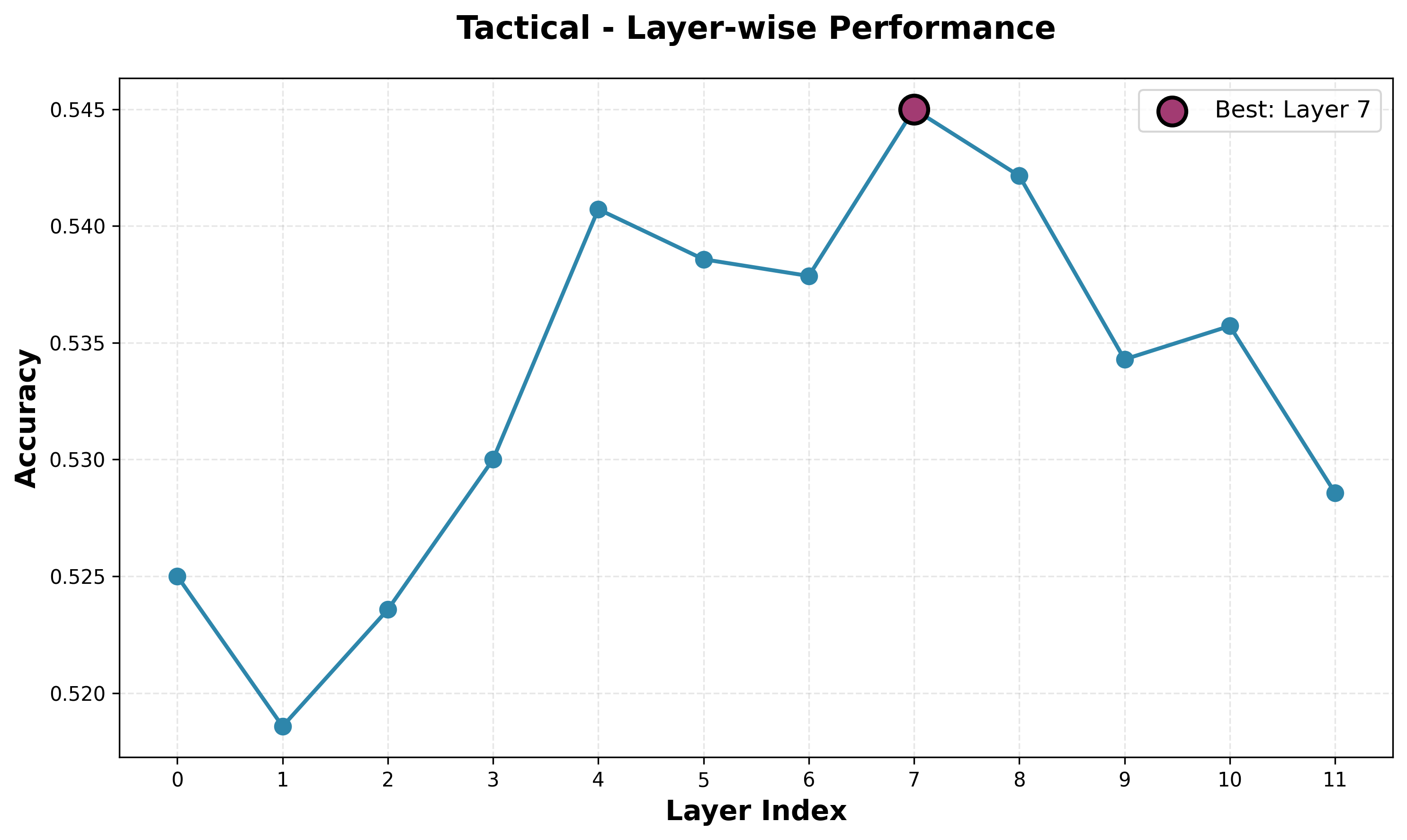
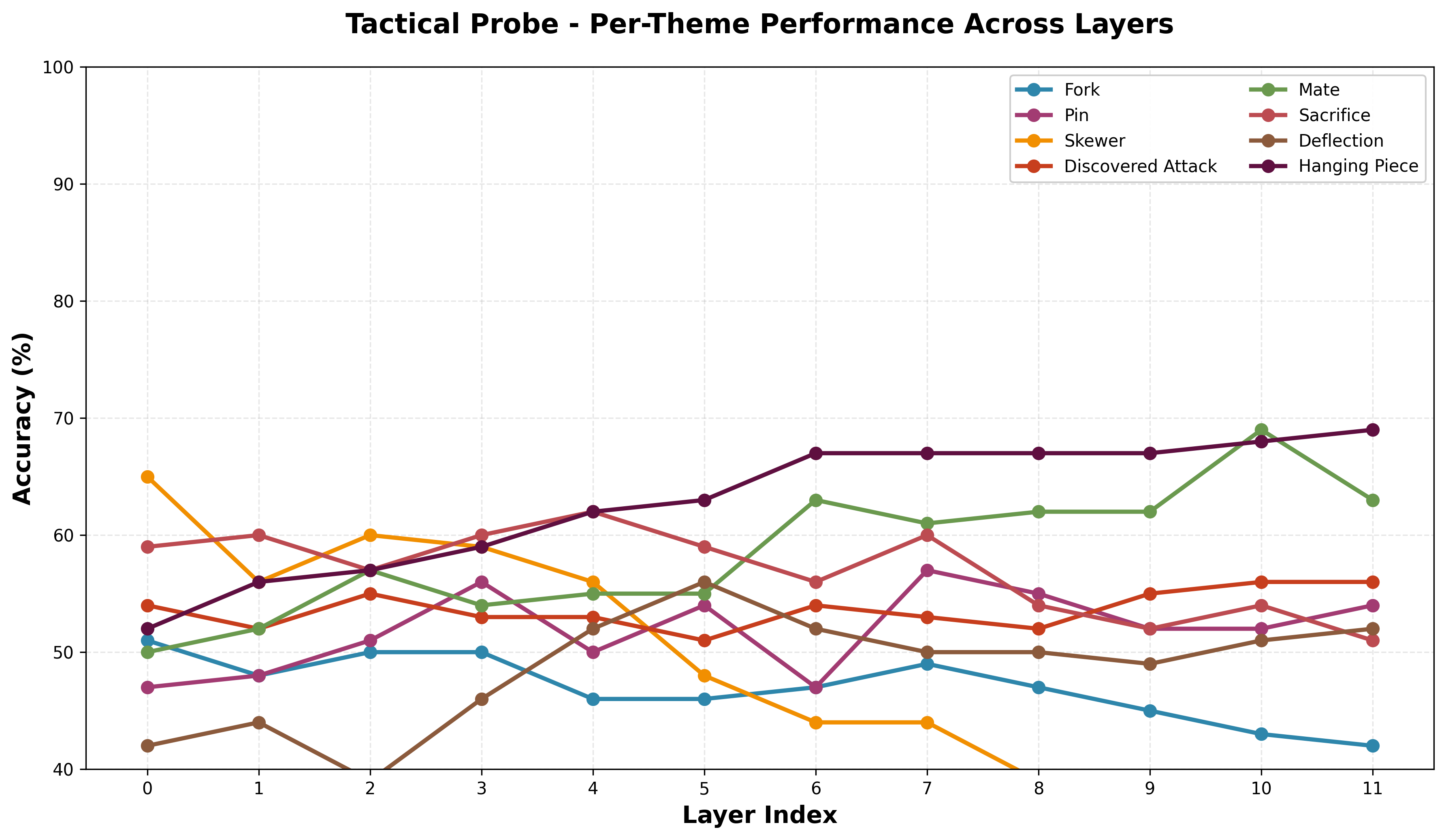
The tactical probes have pretty bad performance and lower performance than I had hoped for. At some point across the layers, each model has above 50% accuracy, meaning it is learning something, but not enough to be significant. In part, I think this can be attributed to the smaller model size, and I will probably try to train a larger model with more data and reevaluate performance. We do, however, see a peak in average performance on a later layer, which fits the narrative that higher-order concepts are strongest represented later in the network. Looking at the per-theme performance, it is important to note that performance looks less smooth and more stochastic across layers compared to other probes, though there is a general upward trend. Different patterns have relatively clearly stronger representations at different points in the network, but it is hard to make a definitive claim about higher or lower order patterns being represented well at different points.
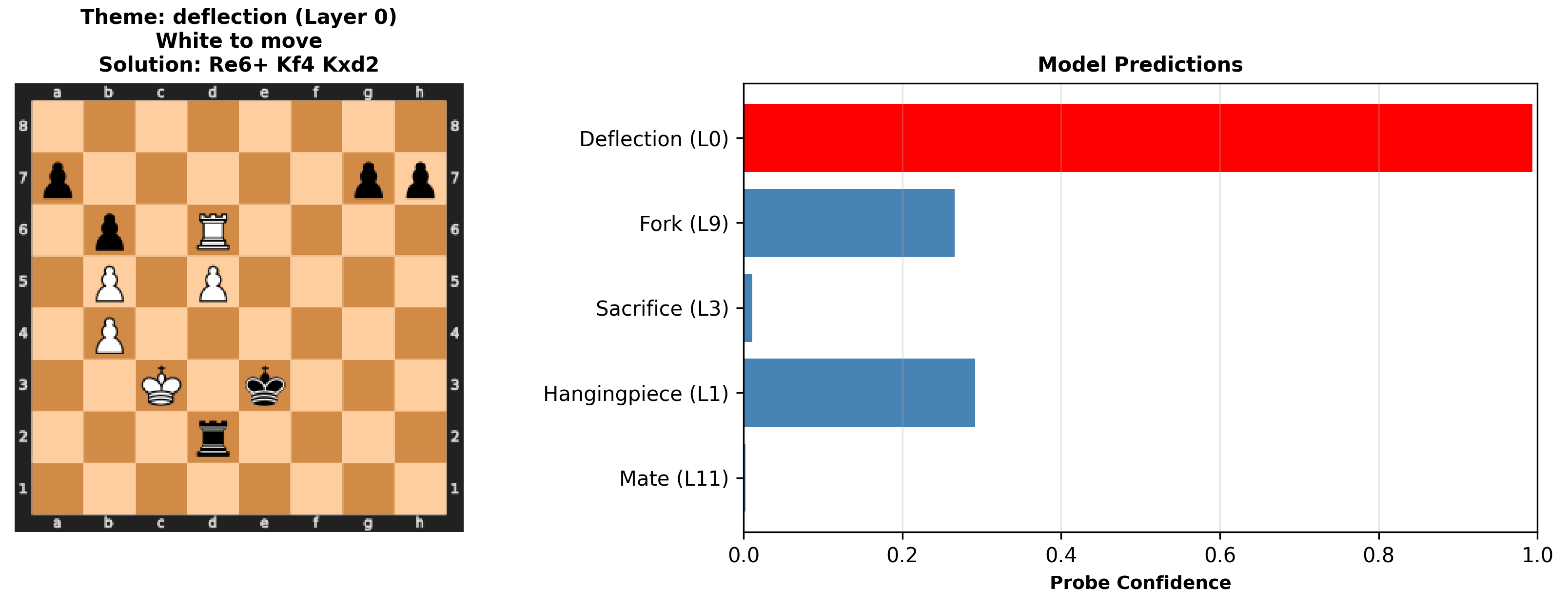
Looking at some examples, we see the model does very well on obvious puzzles, and is even able to discern some more complicated tactics. Note that some puzzles have multiple themes, and while I only display one theme in the title, these themes are correctly used when training and evaluating. However, when a theme is not present we still see some probes detecting tactics. Moreover, the model just completely fails to detect the theme in some puzzles. This seems especially to be the case with longer puzzles, and it may be worth trying to limit the dataset to only a few moves, or even training a different probe for different look ahead distances. Still, I would hope to see the feature for a given tactic present in advance of the given state that has that tactic, as this would show the model has some understanding of not just the game now, but where the game is heading and what moves will be available then.
For a future direction, I would like to test the model's puzzle performance, seeing which moves it takes. I suspect that even though it is identifying themes, it may not be able to actually find the right sequence of moves. I think overall, scaling up training, including model size, data, and train time, may give clearer features, especially for tactics.